Data science project can be a challenging but rewarding process. By following the steps we can use in this blog, you can work through the project in an organized and effective way, and ultimately arrive at a solution to your problem.
Previously, we wrote blogs on many machine learning algorithms (Classification, Predication) as well as many other topics to help you sharpen your knowledge of how machine work. Please kindly visit our site and we would be happy if we got some feedback from you to improve our writing. To see some of them, you can follow the mentioned links.
Dataset is from Kaggle. This is the bank dataset for Credit evaluation whether to grant loan or not.
https://www.kaggle.com/datasets/brycecf/give-me-some-credit-dataset
Disclaimer: This exercise is targeted to audience of all levels including the beginners, so we will be using simple methods, not advanced functions.
Some of concept in this blog are borrowed from lecture note of Data Scientist Nirmal Budhathoki.
This post has been cross-posted from my GitHub page iamdurga.github.io.
Our goal:
For this notebook, we want to perform Exploratory Data Analysis (EDA), learn some data cleaning techniques, handling missing values and etc.
Business Understanding: For the banks, customers going to delinquent or default is a bad news. These are people who are not able to pay their credit. The defaulted loans goes to collection team. This is a loss for bank. Therefore, if we can predict whether a customer will default in next 90 days, then bank can take precautionary actions like interest relief, lower payment plan, extending payoff time etc.
Importing Required Libraries
import pandas as pd
import numpy as np
import joblib
import matplotlib.pyplot as plt
import seaborn as sns
%matplotlib inline
from IPython.display import Image
import warnings
from sklearn.linear_model import LogisticRegression
from sklearn.ensemble import RandomForestClassifier
from sklearn.preprocessing import StandardScaler
from sklearn.model_selection import train_test_split
from sklearn import metrics
from sklearn.metrics import confusion_matrix, classification_report, precision_recall_curve,recall_score
warnings.filterwarnings('ignore')

sns.set(rc={'figure.figsize':(10,8)})
Data Understanding:
Loading Data - We will only load training data for this exercise. You have to download the cs-training.csv from the above link and upload the file into you Google Drive. You can also use the API to read it from kaggle directly. More information on API in this link: https://www.kaggle.com/general/74235
## For now we will load from the drive
dataset = pd.read_csv('cs-training.csv')
## Checking top 5 rows
dataset.head()| Unnamed: 0 | SeriousDlqin2yrs | RevolvingUtilizationOfUnsecuredLines | age | NumberOfTime30-59DaysPastDueNotWorse | DebtRatio | MonthlyIncome | NumberOfOpenCreditLinesAndLoans | NumberOfTimes90DaysLate | NumberRealEstateLoansOrLines | NumberOfTime60-89DaysPastDueNotWorse | NumberOfDependents | |
|---|---|---|---|---|---|---|---|---|---|---|---|---|
| 0 | 1 | 1 | 0.766127 | 45 | 2 | 0.802982 | 9120.0 | 13 | 0 | 6 | 0 | 2.0 |
| 1 | 2 | 0 | 0.957151 | 40 | 0 | 0.121876 | 2600.0 | 4 | 0 | 0 | 0 | 1.0 |
| 2 | 3 | 0 | 0.658180 | 38 | 1 | 0.085113 | 3042.0 | 2 | 1 | 0 | 0 | 0.0 |
| 3 | 4 | 0 | 0.233810 | 30 | 0 | 0.036050 | 3300.0 | 5 | 0 | 0 | 0 | 0.0 |
| 4 | 5 | 0 | 0.907239 | 49 | 1 | 0.024926 | 63588.0 | 7 | 0 | 1 | 0 | 0.0 |
Checking the shape of Dataframe
dataset.shape(150000, 12)Check the data types
dataset.info()
RangeIndex: 150000 entries, 0 to 149999
Data columns (total 12 columns):
 #   Column                                Non-Null Count   Dtype
---  ------                                --------------   -----
 0   Unnamed: 0                            150000 non-null  int64
 1   SeriousDlqin2yrs                      150000 non-null  int64
 2   RevolvingUtilizationOfUnsecuredLines  150000 non-null  float64
 3   age                                   150000 non-null  int64
 4   NumberOfTime30-59DaysPastDueNotWorse  150000 non-null  int64
 5   DebtRatio                             150000 non-null  float64
 6   MonthlyIncome                         120269 non-null  float64
 7   NumberOfOpenCreditLinesAndLoans       150000 non-null  int64
 8   NumberOfTimes90DaysLate               150000 non-null  int64
 9   NumberRealEstateLoansOrLines          150000 non-null  int64
 10  NumberOfTime60-89DaysPastDueNotWorse  150000 non-null  int64
 11  NumberOfDependents                    146076 non-null  float64
dtypes: float64(4), int64(8)
memory usage: 13.7 MB
Observation: All Columns are Numeric, either int or float
Check for Missing Values
dataset.isnull().sum()Unnamed: 0 0
SeriousDlqin2yrs 0
RevolvingUtilizationOfUnsecuredLines 0
age 0
NumberOfTime30-59DaysPastDueNotWorse 0
DebtRatio 0
MonthlyIncome 29731
NumberOfOpenCreditLinesAndLoans 0
NumberOfTimes90DaysLate 0
NumberRealEstateLoansOrLines 0
NumberOfTime60-89DaysPastDueNotWorse 0
NumberOfDependents 3924
dtype: int64Observation: There are two attributes missing some values, lets see the percentage missing.
dataset.isnull().sum() * 100 / len(df)Unnamed: 0 0.000000
SeriousDlqin2yrs 0.000000
RevolvingUtilizationOfUnsecuredLines 0.000000
age 0.000000
NumberOfTime30-59DaysPastDueNotWorse 0.000000
DebtRatio 0.000000
MonthlyIncome 19.820667
NumberOfOpenCreditLinesAndLoans 0.000000
NumberOfTimes90DaysLate 0.000000
NumberRealEstateLoansOrLines 0.000000
NumberOfTime60-89DaysPastDueNotWorse 0.000000
NumberOfDependents 2.616000
dtype: float64dataset.nunique()Unnamed: 0 150000
SeriousDlqin2yrs 2
RevolvingUtilizationOfUnsecuredLines 125728
age 86
NumberOfTime30-59DaysPastDueNotWorse 16
DebtRatio 114194
MonthlyIncome 13594
NumberOfOpenCreditLinesAndLoans 58
NumberOfTimes90DaysLate 19
NumberRealEstateLoansOrLines 28
NumberOfTime60-89DaysPastDueNotWorse 13
NumberOfDependents 13
dtype: int64dataset.duplicated().value_counts()False 150000
dtype: int64dataset['Unnamed: 0'].describe()count 150000.000000
mean 75000.500000
std 43301.414527
min 1.000000
25% 37500.750000
50% 75000.500000
75% 112500.250000
max 150000.000000
Name: Unnamed: 0, dtype: float64Observation: This is just the index field or unique row number , which will not add any value to the modeling. so lets drop it.
dataset.drop(columns = ['Unnamed: 0'], axis=1, inplace = True)dataset.duplicated().value_counts()False 149391
True 609
dtype: int64dataset = dataset.drop_duplicates()dataset.shape(149391, 11)Now lets see how our labels are distributed
dataset['SeriousDlqin2yrs'].value_counts(normalize= True)0 0.933001
1 0.066999
Name: SeriousDlqin2yrs, dtype: float64df['SeriousDlqin2yrs'].value_counts(normalize=True).plot(kind='barh');

Observation: We have roughly 93% NOT Delinquient, and only 7% customers are delinquent. This is classic example of CLASS IMBALANCE.
UNIVARIATE ANALYSIS - ONE VARIABLE AT A TIME
## UNIVARIATE ANALYSIS
# Creating histograms
dataset.hist(figsize=(14,14))
plt.show()
dataset['RevolvingUtilizationOfUnsecuredLines'].describe()count 149391.000000
mean 6.071087
std 250.263672
min 0.000000
25% 0.030132
50% 0.154235
75% 0.556494
max 50708.000000
Name: RevolvingUtilizationOfUnsecuredLines, dtype: float64Observation: The max value is questionable. The revolving utilization means ratio of credit balance/ credit limit, which should always be 0 to 1, since it is ratio. Now lets see how many of such values we have.
len(dataset[(dataset['RevolvingUtilizationOfUnsecuredLines']>1)])3321## Lets see distribution of values that are <= 1
dataset_revUtil_less_than_one= dataset.loc[dataset['RevolvingUtilizationOfUnsecuredLines'] <=1]
sns.displot(data= dataset_revUtil_less_than_one, x= "RevolvingUtilizationOfUnsecuredLines", kde= True);
## since there are 3321 values have issues, its better to treat them as Nulls first and then impute, we can try ffill
dataset['RevolvingUtilizationOfUnsecuredLines'] = dataset['RevolvingUtilizationOfUnsecuredLines'].map(lambda x: np.NaN if x >1 else x)
dataset['RevolvingUtilizationOfUnsecuredLines'].fillna(method='ffill', inplace=True)dataset['RevolvingUtilizationOfUnsecuredLines'].describe()count 149391.000000
mean 6.071087
std 250.263672
min 0.000000
25% 0.030132
50% 0.154235
75% 0.556494
max 50708.000000
Name: RevolvingUtilizationOfUnsecuredLines, dtype: float64dataset['RevolvingUtilizationOfUnsecuredLines'].plot.hist();
We are able to change all the data into 0 to 1 range.
Age
dataset['age'].describe()count 149391.000000
mean 52.306237
std 14.725962
min 0.000000
25% 41.000000
50% 52.000000
75% 63.000000
max 109.000000
Name: age, dtype: float64sns.displot(data = dataset['age'], kde= True);
sns.boxplot(data= dataset['age'])
Using Z Score for Outlier Analysis
dataset['age_zscore'] = (dataset['age'] - dataset['age'].mean())/dataset['age'].std(ddof=0)
dataset.head()| SeriousDlqin2yrs | RevolvingUtilizationOfUnsecuredLines | age | NumberOfTime30-59DaysPastDueNotWorse | DebtRatio | MonthlyIncome | NumberOfOpenCreditLinesAndLoans | NumberOfTimes90DaysLate | NumberRealEstateLoansOrLines | NumberOfTime60-89DaysPastDueNotWorse | NumberOfDependents | age_zscore | |
|---|---|---|---|---|---|---|---|---|---|---|---|---|
| 0 | 1 | 0.766127 | 45 | 2 | 0.802982 | 9120.0 | 13 | 0 | 6 | 0 | 2.0 | -0.496148 |
| 1 | 0 | 0.957151 | 40 | 0 | 0.121876 | 2600.0 | 4 | 0 | 0 | 0 | 1.0 | -0.835686 |
| 2 | 0 | 0.658180 | 38 | 1 | 0.085113 | 3042.0 | 2 | 1 | 0 | 0 | 0.0 | -0.971501 |
| 3 | 0 | 0.233810 | 30 | 0 | 0.036050 | 3300.0 | 5 | 0 | 0 | 0 | 0.0 | -1.514761 |
| 4 | 0 | 0.907239 | 49 | 1 | 0.024926 | 63588.0 | 7 | 0 | 1 | 0 | 0.0 | -0.224518 |
dataset[(dataset['age_zscore'] > 3) | (df['age_zscore'] < -3)].shape(45, 12)condition= dataset[(dataset['age_zscore'] > 3) | (dataset['age_zscore'] < -3)]dataset.drop(condition.index, inplace= True)df.shape(149346, 12)sns.boxplot(data= dataset['age'])
dataset['age'].describe()count 149346.000000
mean 52.292689
std 14.705177
min 21.000000
25% 41.000000
50% 52.000000
75% 63.000000
max 96.000000
Name: age, dtype: float64DEBT RATIO
Debt to income ratio or debt to assets ratio. This is typically 0 to 1, but sometimes it can be higher than 1, meaning person has more debt than income or assets.
dataset['DebtRatio'].describe()count 149346.000000
mean 354.501212
std 2042.133602
min 0.000000
25% 0.177484
50% 0.368253
75% 0.875062
max 329664.000000
Name: DebtRatio, dtype: float64dataset2=dataset[dataset['DebtRatio']>1]['DebtRatio']
dataset26 5710.000000
8 46.000000
14 477.000000
16 2058.000000
25 1.595253
...
149976 60.000000
149977 349.000000
149984 25.000000
149992 4132.000000
149997 3870.000000
Name: DebtRatio, Length: 35115, dtype: float64dataset2.describe()count 35115.000000
mean 1506.721853
std 4000.145613
min 1.000500
25% 42.000000
50% 908.500000
75% 2211.000000
max 329664.000000
Name: DebtRatio, dtype: float64dataset2.plot.box()
Lets make an assumption that Debt to Income ratio should be 0 to 1. Since there are 35,122 data points with Debt ratio higher than 1, instead of dropping them we can make assumption that number with higher than 1 are 100 % Debt ratio so fill them with 1.
dataset['DebtRatio']= dataset['DebtRatio'].apply(lambda x: 1 if x>1 else x)
dataset['DebtRatio']
0 0.802982
1 0.121876
2 0.085113
3 0.036050
4 0.024926
...
149995 0.225131
149996 0.716562
149997 1.000000
149998 0.000000
149999 0.249908
Name: DebtRatio, Length: 149346, dtype: float64df['DebtRatio'].plot.hist()
INCOME
dataset.MonthlyIncome.describe()count 1.201470e+05
mean 6.675649e+03
std 1.439086e+04
min 0.000000e+00
25% 3.400000e+03
50% 5.400000e+03
75% 8.250000e+03
max 3.008750e+06
Name: MonthlyIncome, dtype: float64dataset.MonthlyIncome.isnull().sum()29199dataset.MonthlyIncome.median()5400.0dataset['MonthlyIncome'].fillna(dataset['MonthlyIncome'].median(),inplace=True)dataset.MonthlyIncome.plot.box()
dataset['MonthlyIncome_zscore'] = (dataset['MonthlyIncome'] - dataset['MonthlyIncome'].mean())/dataset['MonthlyIncome'].std(ddof=0)condition= dataset[(dataset['MonthlyIncome_zscore'] > 2) | (dataset['MonthlyIncome_zscore'] < -2)]condition.shape(704, 13)dataset.drop(condition.index, inplace= True)dataset.shape(148642, 13)dataset.MonthlyIncome.plot.box()
dataset.MonthlyIncome.describe()count 148642.000000
mean 6089.029790
std 3775.044698
min 0.000000
25% 3900.000000
50% 5400.000000
75% 7333.000000
max 32250.000000
Name: MonthlyIncome, dtype: float64## If we want bin size of 1000 ,
bins = int((dataset.MonthlyIncome.max() - dataset.MonthlyIncome.min()) / 1000)
print(bins)32dataset.MonthlyIncome.plot.hist(bins=bins)
There are 3 columns giving us information about Late Payments, lets look into them , one at a time.
dataset["NumberOfTimes90DaysLate"].value_counts().sort_index()0 140389
1 5211
2 1551
3 663
4 291
5 130
6 80
7 38
8 21
9 19
10 8
11 5
12 2
13 4
14 2
15 2
17 1
96 5
98 220
Name: NumberOfTimes90DaysLate, dtype: int64plt.xscale('log') ## this is to visualize better if not in log scale it is heavily skewed
dataset["NumberOfTimes90DaysLate"].value_counts().sort_index().plot(kind= 'barh')
dataset["NumberOfTime60-89DaysPastDueNotWorse"].value_counts().sort_index()0 141111
1 5706
2 1116
3 317
4 104
5 34
6 16
7 9
8 2
9 1
11 1
96 5
98 220
Name: NumberOfTime60-89DaysPastDueNotWorse, dtype: int64dataset["NumberOfTime30-59DaysPastDueNotWorse"].value_counts().sort_index()0 124823
1 15953
2 4574
3 1744
4 745
5 341
6 138
7 54
8 25
9 12
10 4
11 1
12 2
13 1
96 5
98 220
Name: NumberOfTime30-59DaysPastDueNotWorse, dtype: int64dataset["NumberOfDependents"].describe()count 144827.000000
mean 0.757338
std 1.114128
min 0.000000
25% 0.000000
50% 0.000000
75% 1.000000
max 20.000000
Name: NumberOfDependents, dtype: float64dataset["NumberOfDependents"].isnull().sum()3815dataset["NumberOfDependents"].plot.box()
dataset['NumberOfDependents'].median()0.0# IMPUTE
dataset['NumberOfDependents'].fillna(dataset['NumberOfDependents'].median(),inplace=True)
dataset["NumberOfDependents"].isnull().sum()0BI-VARIATE ANALYSIS - TWO VARIABLES AT A TIME
SeriousDlqin2yrs Vs. RevolvingUtilizationOfUnsecuredLines
dataset['RevolvingUtilizationOfUnsecuredLines'].groupby(dataset.SeriousDlqin2yrs).mean().plot(kind='bar', color=['blue', 'green'])
plt.ylabel('Ratio')
plt.title('Distribution of RevolvingUtilizationOfUnsecuredLines with label')
Text(0.5, 1.0, 'Distribution of RevolvingUtilizationOfUnsecuredLines with label')
Observation: Delinquent customers got almost twice the utilization of unsecured lines
SeriousDlqin2yrs Vs. Age
dataset['age'].groupby(dataset.SeriousDlqin2yrs).mean().plot(kind='bar', color=['blue', 'green'])
plt.ylabel('Age')
plt.title('Distribution of Age with label')
Text(0.5, 1.0, 'Distribution of Age with label')
Observation: On average lower aged customers are more delinquent
SeriousDlqin2yrs Vs. DebtRatio
dataset['DebtRatio'].groupby(dataset.SeriousDlqin2yrs).mean().plot(kind='bar', color=['blue', 'green'])
plt.ylabel('DebtRatio')
plt.title('Distribution of Debt Ratio with label')
Text(0.5, 1.0, 'Distribution of Debt Ratio with label')
Observation: ??? Ask to Class
SeriousDlqin2yrs Vs. MonthlyIncome
dataset['MonthlyIncome'].groupby(dataset.SeriousDlqin2yrs).mean().plot(kind='bar', color=['blue', 'green'])
plt.ylabel('Monthly Income')
plt.title('Distribution of Monthly Income with label')
Text(0.5, 1.0, 'Distribution of Monthly Income with label')
Observation: ??? Ask to Class
MULTI VARIATE ANALYSIS - more than two variables at a time, we will do correlation heatmap for this.
## First lets drop the z_score columns we create to remove outliers
dataset=dataset.drop(['age_zscore', 'MonthlyIncome_zscore'], axis=1)
dataset.columnsIndex(['SeriousDlqin2yrs', 'RevolvingUtilizationOfUnsecuredLines', 'age',
'NumberOfTime30-59DaysPastDueNotWorse', 'DebtRatio', 'MonthlyIncome',
'NumberOfOpenCreditLinesAndLoans', 'NumberOfTimes90DaysLate',
'NumberRealEstateLoansOrLines', 'NumberOfTime60-89DaysPastDueNotWorse',
'NumberOfDependents'],
dtype='object')corr = dataset.corr()
#sns.heatmap(corr) # simple but shows more noisy plot, adding mask to only see half is better
mask = np.zeros_like(corr)
mask[np.triu_indices_from(mask)] = True
with sns.axes_style("white"):
f, ax = plt.subplots(figsize=(10, 8))
ax = sns.heatmap(corr, mask=mask, square=True)
above figure shows that age and SeriousDlqin2yrs are highly correlated similarly NumberOfTimes90DaysLate and NumberOfTime30-59DaysPastDueNotWorse are less correlated. In the same way we can estimate the relationship between different attributes.
FEATURE ENGINEERING
What are some of the additional features we can create or drive from given attributes?
- We have monthly income and total dependents, we can derive income per person
- We have Debt to Income ratio so we can get total debt
- From 1 & 2, we can get monthly balance
- We can also sum all the dues , 30- 59 days, 60- 89 days, and 90 days
Let's add these 4 new features for now.
# Income per person
dataset['Income_per_person'] = dataset['MonthlyIncome']/(dataset['NumberOfDependents']+1)
# Monthly Debt
dataset['Monthly_debt'] = dataset['DebtRatio']*dataset['MonthlyIncome']
# Monthly Balance
dataset['Monthly_balance'] = dataset['MonthlyIncome'] - dataset['Monthly_debt']
# Total number of DUEs
dataset['Total_number_of_dues'] = dataset['NumberOfTime30-59DaysPastDueNotWorse']+dataset['NumberOfTime60-89DaysPastDueNotWorse']+dataset['NumberOfTimes90DaysLate']
dataset.head()| SeriousDlqin2yrs | RevolvingUtilizationOfUnsecuredLines | age | NumberOfTime30-59DaysPastDueNotWorse | DebtRatio | MonthlyIncome | NumberOfOpenCreditLinesAndLoans | NumberOfTimes90DaysLate | NumberRealEstateLoansOrLines | NumberOfTime60-89DaysPastDueNotWorse | NumberOfDependents | |
|---|---|---|---|---|---|---|---|---|---|---|---|
| 0 | 1 | 0.766127 | 45 | 2 | 0.802982 | 9120.0 | 13 | 0 | 6 | 0 | 2.0 |
| 1 | 0 | 0.957151 | 40 | 0 | 0.121876 | 2600.0 | 4 | 0 | 0 | 0 | 1.0 |
| 2 | 0 | 0.658180 | 38 | 1 | 0.085113 | 3042.0 | 2 | 1 | 0 | 0 | 0.0 |
| 3 | 0 | 0.233810 | 30 | 0 | 0.036050 | 3300.0 | 5 | 0 | 0 | 0 | 0.0 |
| 5 | 0 | 0.213179 | 74 | 0 | 0.375607 | 3500.0 | 3 | 0 | 1 | 0 | 1.0 |
MODEL BUILDING
Before we start modeling, we need to make sure what evaluation metrics to use. Since we have imbalanced data set, we will be using Precision- Recall, and f1-score for evaluation.
Class 1: (YES) : Delinquent Customers
Class 2: (NO): Non- Delinquent Customers
Here Class of Interest is positive class- which is Class 1. Lets discuss what could be more costly for business- whether False Positives or False Negatives.
If we predict customers will delinquent, but they are not. This means False Positives, because we falsely predicted positive class.
If we predict customers will NOT delinquent, but in reality they did. This means False Negatives, because we falsely predicted negative class.
From bank's perspective, False Negative is more costly, because we miss to predict the customers who will delinquent. Since False Negatives matter more, we should aim to reduce FNs, that means RECALL will be more important that PRECISION.
Precision = TP / TP + FP
Recall = TP / TP + FN
Steps to follow:
- Split the data into train and test set (lets take 70-30 split)
- Scale the data ( also called normalize): we can pick StandardScaler or MinMaxScaler
- Try 3 different models: Logistic Regression, RandomForest, XGBoost
- Compare the evaluation metrics
- Pick the best performing and generalized model
## TRAIN AND TEST SPLIT 70 to 30 percent

X = dataset.drop(columns=['SeriousDlqin2yrs'])
y = dataset['SeriousDlqin2yrs']
X_train, X_test, y_train, y_test = train_test_split(X, y,stratify= y,random_state=42,shuffle=True,test_size=0.3)
print('Shape of training data', X_train.shape)
print('-'*40)
print('Shape of test data', X_test.shape)
print('-'*40)
Shape of training data (104049, 10)
----------------------------------------
Shape of test data (44593, 10)
----------------------------------------
## SCALE THE DATA, we will use standard scaler
sc= StandardScaler()
X_train_scaled=sc.fit_transform(X_train)
X_train_scaled=pd.DataFrame(X_train_scaled, columns=X.columns)
# Transform on test data
X_test_scaled=sc.transform(X_test)
X_test_scaled=pd.DataFrame(X_test_scaled, columns=X.columns)X_train_scaled.head()| RevolvingUtilizationOfUnsecuredLines | age | NumberOfTime30-59DaysPastDueNotWorse | DebtRatio | MonthlyIncome | NumberOfOpenCreditLinesAndLoans | NumberOfTimes90DaysLate | NumberRealEstateLoansOrLines | NumberOfTime60-89DaysPastDueNotWorse | NumberOfDependents | |
|---|---|---|---|---|---|---|---|---|---|---|
| 0 | -0.027215 | 1.475614 | -0.102208 | -1.283644 | 0.112021 | -0.289289 | -0.062012 | -0.912388 | -0.055610 | 0.239036 |
| 1 | -0.027219 | 0.386825 | -0.102208 | -1.137202 | -0.183511 | 0.099620 | -0.062012 | -0.912388 | -0.055610 | -0.666237 |
| 2 | -0.023049 | -0.429767 | -0.102208 | -0.397614 | 0.367459 | -0.094834 | 0.201595 | -0.015583 | 0.209069 | 1.144309 |
| 3 | -0.024338 | 0.727071 | 0.159529 | 1.496206 | -0.183511 | 0.294075 | -0.062012 | -0.015583 | -0.055610 | -0.666237 |
| 4 | -0.025999 | 1.067318 | -0.102208 | 0.137173 | -0.285739 | -0.483743 | -0.062012 | 0.881221 | -0.055610 | -0.666237 |
# Creating metric function
# Metrics to evaluate the model
def metrics_score(actual, predicted):
    print(classification_report(actual, predicted))
    cm = confusion_matrix(actual, predicted)
    plt.figure(figsize=(8,5))

    sns.heatmap(cm, annot=True,  fmt='.2f', xticklabels=['Not Delinquent', 'Delinquent'], yticklabels=['Not Delinquent', 'Delinquent'])
    plt.ylabel('Actual')
    plt.xlabel('Predicted')
plt.show()X_train_scaled.isnull().sum()RevolvingUtilizationOfUnsecuredLines 0
age 0
NumberOfTime30-59DaysPastDueNotWorse 0
DebtRatio 0
MonthlyIncome 0
NumberOfOpenCreditLinesAndLoans 0
NumberOfTimes90DaysLate 0
NumberRealEstateLoansOrLines 0
NumberOfTime60-89DaysPastDueNotWorse 0
NumberOfDependents 0
dtype: int64# Fitting logistic regression model
lg=LogisticRegression(random_state=42, class_weight='balanced')
lg.fit(X_train_scaled,y_train)LogisticRegression(class_weight='balanced', random_state=42)# Checking the performance on the training data
y_pred_train = lg.predict(X_train_scaled)
metrics_score(y_train, y_pred_train) precision recall f1-score support
0 0.97 0.79 0.87 97071
1 0.19 0.66 0.29 6978
accuracy 0.78 104049
macro avg 0.58 0.72 0.58 104049
weighted avg 0.92 0.78 0.83 104049
# Checking the performance on the test dataset
y_pred_test = lg.predict(X_test_scaled)
metrics_score(y_test, y_pred_test)
precision recall f1-score support
0 0.97 0.78 0.86 41603
1 0.19 0.72 0.30 2990
accuracy 0.77 44593
macro avg 0.58 0.75 0.58 44593
weighted avg 0.92 0.77 0.83 44593
# Printing the coefficients of logistic regression
cols=X.columns
coef_lg=lg.coef_
pd.DataFrame(coef_lg,columns=cols).T.sort_values(by = 0,ascending = False)| 0 | |
|---|---|
| NumberOfTimes90DaysLate | 2.297865 |
| NumberOfTime30-59DaysPastDueNotWorse | 2.134538 |
| NumberOfTime60-89DaysPastDueNotWorse | 0.543397 |
| NumberOfDependents | 0.097003 |
| DebtRatio | 0.094698 |
| NumberRealEstateLoansOrLines | 0.062493 |
| NumberOfOpenCreditLinesAndLoans | 0.011010 |
| RevolvingUtilizationOfUnsecuredLines | -0.012984 |
| MonthlyIncome | -0.147554 |
| age | -0.450574 |
# Predict_proba gives the probability of each observation belonging to each class
y_scores_lg=lg.predict_proba(X_train_scaled)
precisions_lg, recalls_lg, thresholds_lg = precision_recall_curve(y_train, y_scores_lg[:,1])

# Plot values of precisions, recalls, and thresholds
plt.figure(figsize=(10,7))
plt.plot(thresholds_lg, precisions_lg[:-1], 'b--', label='precision')
plt.plot(thresholds_lg, recalls_lg[:-1], 'g--', label = 'recall')
plt.xlabel('Threshold')
plt.legend(loc='upper left')
plt.ylim([0,1])
plt.show()
## Intersection of Precision and Recall is Optimum threshold
optimal_threshold=.78
y_pred_train = lg.predict_proba(X_train_scaled)

metrics_score(y_train, y_pred_train[:,1]>optimal_threshold)
precision recall f1-score support
0 0.95 0.98 0.96 97071
1 0.49 0.25 0.33 6978
accuracy 0.93 104049
macro avg 0.72 0.62 0.65 104049
weighted avg 0.92 0.93 0.92 104049
optimal_threshold=.78
y_pred_test = lg.predict_proba(X_test_scaled)
metrics_score(y_test, y_pred_test[:,1]>optimal_threshold)
precision recall f1-score support
0 0.95 0.97 0.96 41603
1 0.42 0.33 0.37 2990
accuracy 0.92 44593
macro avg 0.69 0.65 0.66 44593
weighted avg 0.92 0.92 0.92 44593
Observation:
- The model is giving similar performance on the test and train data i.e. the model is giving a generalized performance.
- The precision of the test data has increased significantly while at the same time, the recall has decreased, which is to be expected while adjusting the threshold.
- Since RECALL is important for us as discussed abaove before we began model building, we CANNOT use higher threshold to lose the recall.
- The average recall and precision for the model are good but let's see if we can get better performance using other algorithms.
Remember our goal is to have better Recall
# Fitting the Random Forest classifier on the training data
rf_estimator = RandomForestClassifier(class_weight = {0: 0.93, 1: 0.07}, random_state = 42) ## class weight comes from initial class distribution
rf_estimator.fit(X_train_scaled, y_train)
RandomForestClassifier(class_weight={0: 0.93, 1: 0.07}, random_state=42)# Checking performance on the training data
y_pred_train_rf = rf_estimator.predict(X_train)
metrics_score(y_train, y_pred_train_rf) precision recall f1-score support
0 0.97 0.65 0.78 97071
1 0.13 0.72 0.22 6978
accuracy 0.66 104049
macro avg 0.55 0.68 0.50 104049
weighted avg 0.91 0.66 0.74 104049
# Checking performance on the testing data
y_pred_test_rf = rf_estimator.predict(X_test)
metrics_score(y_test, y_pred_test_rf)
precision recall f1-score support
0 0.97 0.65 0.78 41603
1 0.13 0.72 0.22 2990
accuracy 0.65 44593
macro avg 0.55 0.69 0.50 44593
weighted avg 0.91 0.65 0.74 44593
You can uncomment and run below cell once to find the best model using GridSearch. I added the code to save the model into the physical drive after finding the best model. So it can be commented again to save the runtime.
## RF with GRIDSEARCH- It will be computationally costly but we shall get better model
# For tuning the model-- Dont run again
# from sklearn.model_selection import StratifiedKFold
# from sklearn.model_selection import GridSearchCV

# skf = StratifiedKFold(n_splits=5, shuffle=True, random_state=5)

# rf = RandomForestClassifier(n_estimators=100, n_jobs=-1, random_state=42,
#                             class_weight='balanced')
# parameters = {'max_features': [1, 2, 4], 'min_samples_leaf': [3, 5, 7, 9], 'max_depth': [5,10,15]}
# rf_grid_search = GridSearchCV(rf, parameters, n_jobs=-1, scoring='roc_auc', cv=skf, verbose=True)
# rf_grid_search = rf_grid_search.fit(X_train, y_train)

# ## SAVING MODEL AS PICKLE FILE, SO you can simply load it in future
# model_save_name = '/content/drive/MyDrive/givemecredit_bestmodel.pkl'
# joblib.dump(rf_grid_search.best_estimator_, model_save_name)
## load the pre-trained model from physical drive
model_save_name = '/content/drive/MyDrive/givemecredit_bestmodel.pkl'
loaded_model = joblib.load(model_save_name)
# Checking performance on the testing data
y_pred_test= loaded_model.predict(X_test)
metrics_score(y_test, y_pred_test)
precision recall f1-score support
0 0.98 0.84 0.90 41603
1 0.24 0.71 0.36 2990
accuracy 0.83 44593
macro avg 0.61 0.77 0.63 44593
weighted avg 0.93 0.83 0.86 44593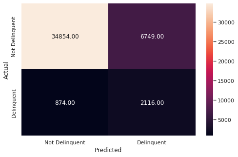
importances = loaded_model.feature_importances_
columns = X.columns
importance_df = pd.DataFrame(importances, index = columns, columns = ['Importance']).sort_values(by = 'Importance', ascending = False)
plt.figure(figsize = (13, 13))
sns.barplot(importance_df.Importance, importance_df.index);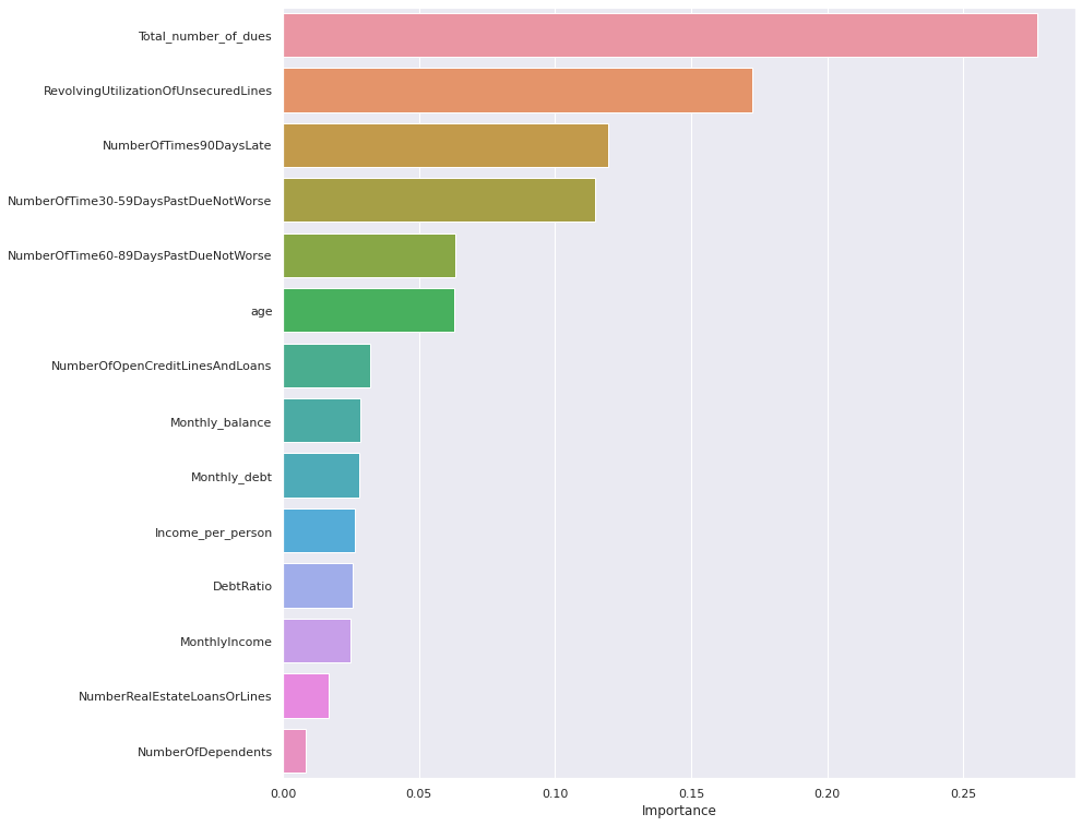
Conclusion:
With Grid Search and 5 fold Cross Validation, we were able to find best model with Training Accuracy of 84% and Test Accuracy of 83% , since both training and test accuracy are similar, our model is generalized. We were also able to maintain the Recall for positive class (Delinquent Customers) around 71%. So compared to all the models we tried, this is the best one to pick.
More things you can try:
- Trying more models: SVMs, and Boosting Models could be other options to try
- Balancing the class- with some sampling techniques and try again
- Additional Feature Engineering