Intro to OpenCV for Image Processing with Python

OpenCV is a multi-platform Image Processing tool which provides lots of algorithms and processes. This notebook was written in 2019 by me when I was just learning, and I missed to add the author of images used from the internet. All images are taken from the internet and credit goes to original authors.

Contains

• Introduction
• Image Representation
• Image Channels
• Image Transforms
• Image Masking
• Image Filtering
• Edge Detection
• Hough Transform
• Haar Cascade for Face Detection

Introduction

• OpenCV was written and originally used on C++ but now, it can be used in Java, Android, C# as well as Unity3D.
• OpenCV can almost do every image processing tasks like filtering, edge detection, transforming, thresholding, video capturing, contour detection and so on.
• Installation: pip install opencv-python or install using whl file
• We will import OpenCv as import cv2

Image Representation

• Image as digital, is stored as array of pixels(Picture Elements) and can be viewed as 2d plot.
• Image has channels, RGB means Red, Green and Blue respectively. Grayscale image has one channel only.
• Each pixel values will be on the range of 0 to 255, if image is 8bit. 0 means the leas intensity of the pixel and 255 represents the maximum intensity of the pixel.
• Shape of image is determined by rows/columns present in it.
• A RGB image of dimension 100 by 100 will contain 3000 pixels(100 100 3)
• We can read image using simple image = cv2.imread(imagepath, colorspace). Here colorspace is a flag 0 or 1. 0 is Grayscale and 1 is RGB.
• A image stores pixels on bits value. A Grayscale image will contain 8 bits pixels.(i.e. one pixel value ranges from 0 to 255 which is 2^8 - 1).

Image Channels

• Image can have at least 1 channel(i.e grayscale)
• RGB image have 3 channels i.e Red, Green, Blue
• Grayscale image have only one color channel i.e Black
• Storage required for image can be calculated as [(Height in pixels) x (length in pixels) x (bit depth)] / 8 / 1024 = image size in kilobytes (KB) ex. RGB image of 100 by 100 allocates at most 37kb
• We can view each channel of image just like numpy array accessing. Ex. for a BGR image, we can get Blue channel as blue_channel = image[::0]
• Converting colorspace on RGB can be done on OpenCv using cv2.cvtColor(image, cv2.COLOR_RGB). OpenCv allows lots of colorspaces like HSV, RGBA etc.

Image Transforms

• Since image can be taken as geometrical shape, we can apply basic geometrical transformations like rotation, zooming etc
• While zooming, we add pixel values(ex. avg. of two pixels)
• While shrinking, we remove pixels(ex. add avg. of two pixels and remove consecutive)
• Resizing image on OpenCv can be done using code: cv2.resize(image, (shape), (ratios))

Image Thresholding

• Thresholding a image converts image pixels into certain values based on the limit of pixels.
• On OpenCv we can threshold image using code:cv2.threshold(image, lower_range, high_range, value)
• Additionally we have Binary thresholding and Otsu as well.

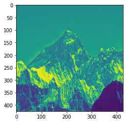
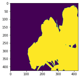
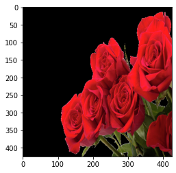
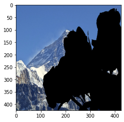
Image Masking

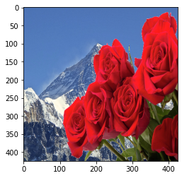
• Masking an image with some filter or mask.
• Adding some image in front of some other image.
• Removing background from image or moving object to other background.
• This can be done after we remove the background pixel from masking image.
• Note that black color must be the background or we must convert it. Because adding black pixels to any other pixels won't affect.

Image filtering

• Image filtering have huge importance on Computer Vision.
• Image filtering uses the concept of image convolution.
• Convolution process uses a small filter(window or kernel) to run over entire image and does elementwise multiplication and sum all.
• Popular image filtering filters are low-pass and high-pass.
• Image filtering applications includes: image averaging, image sharpening, image blurring, edge detection etc
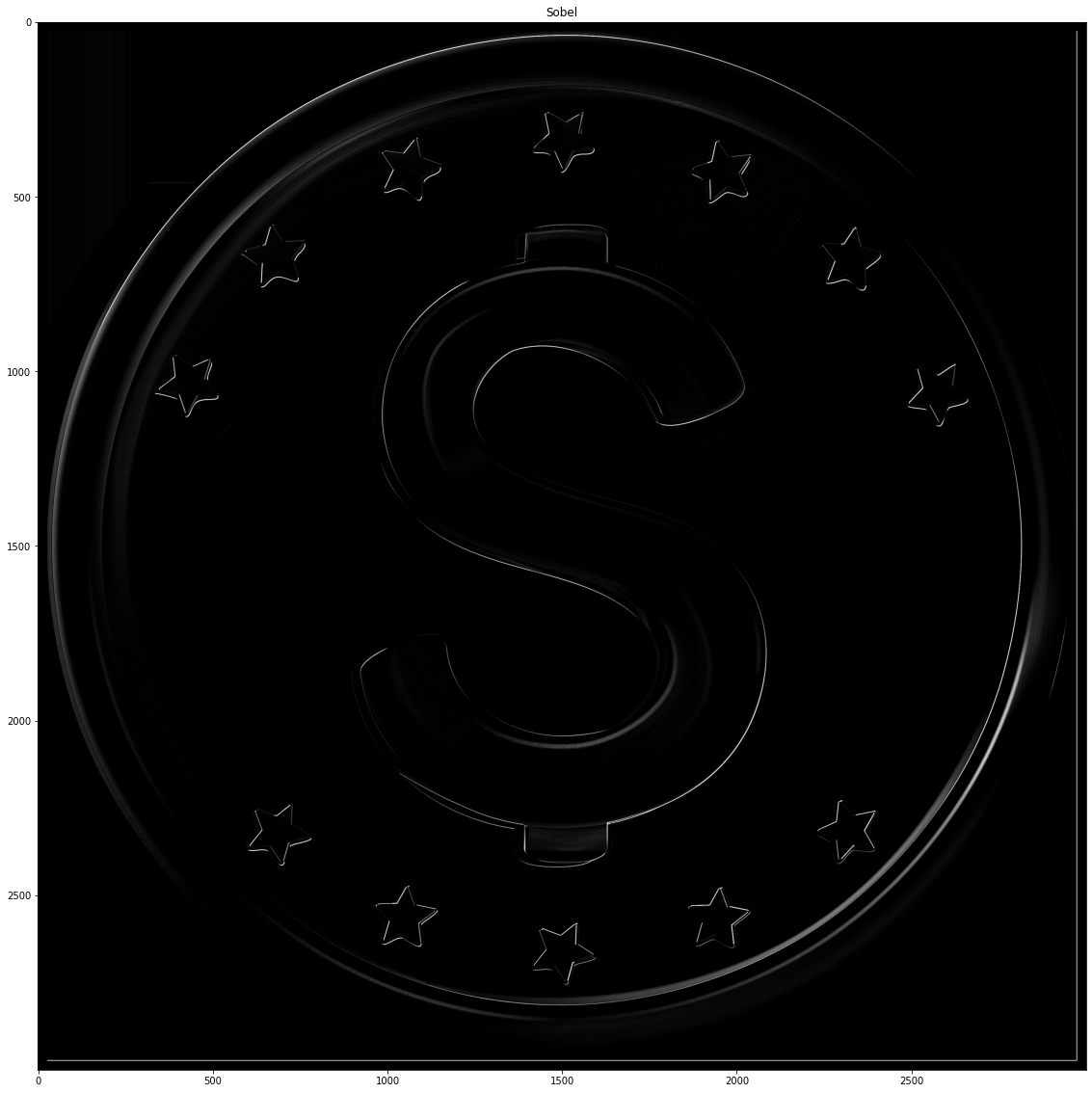
• One of popular filter is Sobel filter done for edge detection.
• High-pass are for sharpening image, enhance features and finding edges.
• Filters are convolutional kernels, ex [[0 -1 0] [-1 4 -1] [0 -1 0]]. Finds change between current and neighbor pixels.
• If output of convolution is 0 or its -ve then its darken else brighter.
• Example of edge detection using high-pass filter:
  
  High-pass filtering image
• Convolution process:
  
  Inside Grayscale image

High pass vs low pass filters

• High-pass are for sharpening image, enhance features and finding edges.
• Filters are convolutional kernels, ex [[0 -1 0] [-1 4 -1] [0 -1 0]]. Finds change between current and neighbor pixels.
• If output of convolution is 0 then no change if its -ve then its darken else brighter.
• For horizontal use ex [[-1 2 -1] [0 0 0] [-1 2 -1]].
• Low pass filters are used for image smoothing and blurring purposes.

Edge Detection

• High-pass filters like Sobel filer is used for convolution process,
• Edge Detection is used to detect objects and many other ROI extraction of images,
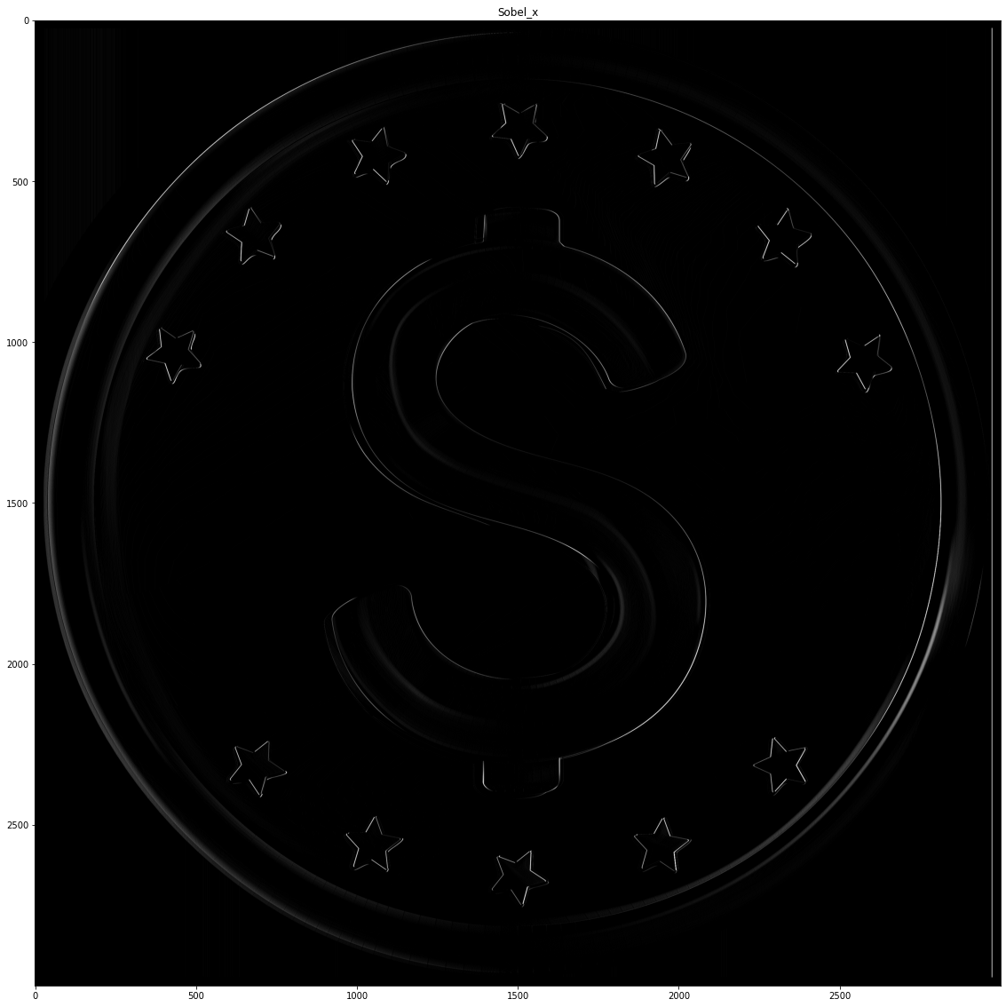
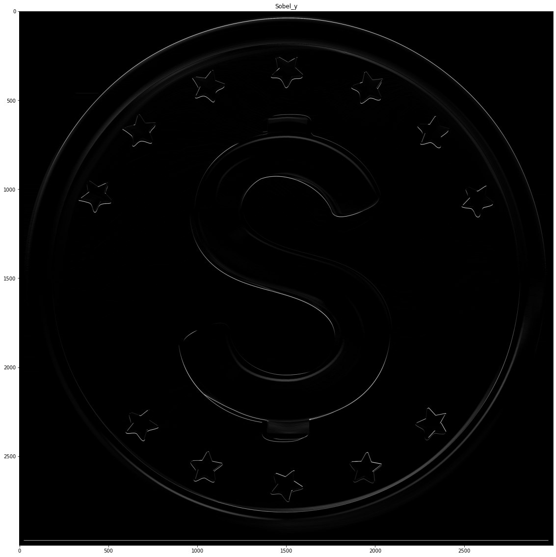
• Sobel filter for detecting horizontal line is [[ -1, 0, 1], [ -2, 0, 2], [ -1, 0, 1]] and known as called sobel_x.
• Sobel filter for detectin vertical line is [[ -1, -2, -1], [ 0, 0, 0], [ 1, 2, 1]] and known as sobel_y.
• Applications of Edge Detection includes extracting border of image,
• Sobel filters can be written using simple numpy array,
• We can apply any 2D filters using code cv2.filter2D(image, depth, kernel) . Kernel should be square array.
• Even better edge detection we can use Canny Edge Detection method.

Canny edge detector

Combination of processes:

• Noise filteration using Gaussian Blur
• Then Sobel filters
• Uses NMS for isolate strongest edges
• Hysteresis thresholding for best edges
• Can be implemented using cv2.Canny(stripes, low, high)

Hough Transform

• Most popular line detection algorithm.
• Can even detect other geometrical shapes like circle, ellipse etc
• A line can be represented as y = mx+c or in parametric form, z = x cos(theta) + y cos(theta) where z is perpendicular distance from origin to line. 'theta' is angle formed by perpendicular line to line.
• Other shapes can be detected using their respective equations
• Applications includes finding geometrical shapes like lines on image
• Can be implemented using cv2.HoughLinesP(canny_img, rho, theta, threshold, np.array([]), max_line_length, max_line_gap)

Haar Cascade for Face detection

• Haar cascade extracts features from images using a kind of filter, similar to the concept of the convolutional kernel
• These are pre-trained XML files which gives the bounding box coordinates of detected face.

Contours

• Contours are simple curves that are joined around a object of same color or intensity.
• For example if we want to extract a edges of bottle, the contour curve will be around the bottle edges only.
• On OpenCv, contour can be drawn easily extracted and drawn.

YOLO(You Only Look Once)

• Introduction
• Setup
• Implementation

Introduction

• Original Paper on https://arxiv.org/abs/1506.02640
• Uses COCO Dataset of 80 classes
• YOLO is currently the most fastest object detection concept currently and can be used on Real Time also

Setup

• We will use pretrained model, and labels
• We can use YOLO Pretrained model by downloading weights from https://pjreddie.com/media/files/yolov3.weights
• We can use configuration from https://github.com/pjreddie/darknet/blob/master/cfg/yolov3.cfg
• We can use COCO Dataset labels from https://github.com/pjreddie/darknet/blob/master/data/coco.names
• YOLO is simple to setup and can be used from even OpenCV

Implementation

• Simple functions of OpenCv can be used to implement YOLO
• We can make a DNN of YOLO using config file from code:

#create the DNN with existing weights and configurations
net = cv2.dnn.readNet('yolov3.weights', 'yolov3.cfg')
#get the layer names
layer_names = net.getLayerNames()
#get o/p layer
output_layers = [layer_names[i[0] - 1] for i in net.getUnconnectedOutLayers()]

• Then we will have to get blob from image and pass it to YOLO model of input shape

#get blob from img..img, scaleFactor, size, means of channel, RGB?
blob = cv2.dnn.blobFromImage(img, 0.00392, (416, 416), (0, 0, 0), True, crop = False)         
#send image to input layer
net.setInput(blob)       
#get output of model
outs = net.forward(output_layers)

• Output of model will contain center coo., height, width, class ids, prediction scores
• We will used NMS(Non Max Suppression) to eliminate multiple bounding boxes around same object

Imports and Image Reading

# import dependencies
import cv2
import numpy as np
import matplotlib.pyplot as plt

#check versions
print(cv2.__version__)

4.5.2

# read image
fg = cv2.imread('(https://q-viper.github.io/assets/intro_opencv/petal.jpg', 1) # 1 reads as BGR 0 reads as Grayscale
fg = cv2.resize(fg, (425, 425))

#shape of image
print(fg.shape)

#show image
cv2.imshow('fg', fg)
cv2.waitKey() # wait for milisecond
cv2.destroyAllWindows()

(425, 425, 3)

print(fg.reshape(1, -1))

[[255 255 255 ... 255 255 255]]

img = cv2.imread('(https://q-viper.github.io/assets/intro_opencv/everest.jpg')

plt.imshow(cv2.cvtColor(img, cv2.COLOR_BGR2GRAY).T)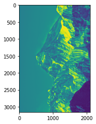

Image Channels

# showing using matplotlib is easy way
plt.imshow(np.array(fg))
plt.title('BGR image')
plt.show()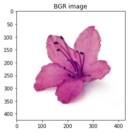

OpenCv reads image as BGR format but matplotlib reads as RGB so we need to convert BGR to RGB

# Color changing
rgb_fg = cv2.cvtColor(fg, cv2.COLOR_BGR2RGB)
plt.imshow(rgb_fg)
plt.title('RGB image')
plt.show()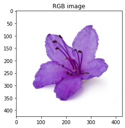

# lets see image channels

red = np.zeros_like(rgb_fg).astype(np.uint8) 
red[:,:,0]=rgb_fg[:,:,0] # red channel

plt.imshow(red) 
plt.show()

green = np.zeros_like(rgb_fg).astype(np.uint8) 
green[:,:,1]=rgb_fg[:,:,1] # green channel

plt.imshow(green) 
plt.show()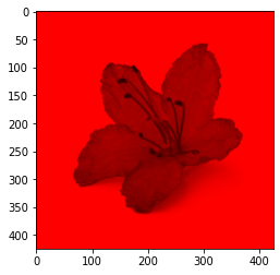

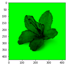
Image Transform

gray_fg = cv2.cvtColor(fg, cv2.COLOR_BGR2GRAY)
# Image Transform
rows,cols = gray_fg.shape

M = cv2.getRotationMatrix2D((cols/2,rows/2),40,1)
dst = cv2.warpAffine(fg,M,(cols,rows))

plt.imshow(dst)
plt.show()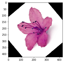

Image Masking

# lets read a pyramid image
pyramid = cv2.imread('(https://q-viper.github.io/assets/intro_opencv/pyramid.jpg', 1)

#reshape pyramid to shape of flag
print(pyramid.shape)

pyramid = cv2.resize(pyramid, (425, 425))

rgb_pyramid = cv2.cvtColor(pyramid, cv2.COLOR_BGR2RGB)
plt.imshow(rgb_pyramid)
plt.show()

(417, 471, 3)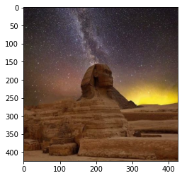

# convert both fg and pyramid into grayscale

gray_fg = cv2.cvtColor(rgb_fg, cv2.COLOR_BGR2GRAY)
gray_pyramid = cv2.cvtColor(rgb_pyramid, cv2.COLOR_BGR2GRAY)

plt.imshow(gray_fg)
plt.show()

plt.imshow(gray_pyramid)
plt.show()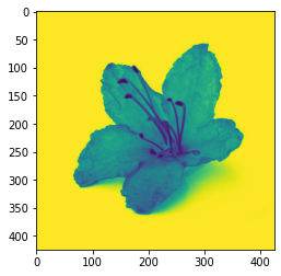

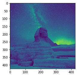
# create a mask of flag

lv = np.array([0, 0, 0])
hv = np.array([220, 220, 220])

mask = cv2.inRange(fg, lv, hv)
plt.imshow(mask)
plt.show()

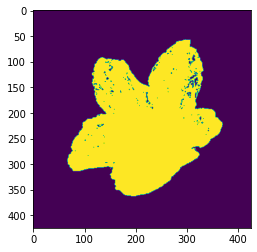
masked_img = rgb_fg.copy()
masked_img[mask != 255] = [0, 0, 0]
plt.imshow(masked_img)
plt.show()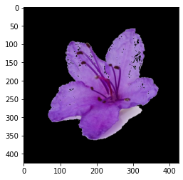

bg_cpy = rgb_pyramid.copy()
bg_cpy[mask == 255] = [0, 0, 0]

plt.imshow(bg_cpy)
plt.show()

final = bg_cpy + masked_img
plt.imshow(final)
plt.show()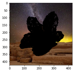

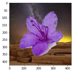
All Codes

## Stackking up

# read image
fg = cv2.imread('(https://q-viper.github.io/assets/intro_opencv/rose.jpg', 1) # 1 reads as BGR 0 reads as Grayscale
fg = cv2.resize(fg, (425, 425))

# Color changing
rgb_fg = cv2.cvtColor(fg, cv2.COLOR_BGR2RGB)
plt.imshow(rgb_fg)
plt.title('RGB image')
plt.show()

# lets read a pyramid image
pyramid = cv2.imread('(https://q-viper.github.io/assets/intro_opencv/everest.jpg', 1)

#reshape pyramid to shape of flag
print(pyramid.shape)

pyramid = cv2.resize(pyramid, (425, 425))

rgb_pyramid = cv2.cvtColor(pyramid, cv2.COLOR_BGR2RGB)
plt.imshow(rgb_pyramid)
plt.show()

# convert both flag and pyramid into grayscale

gray_fg = cv2.cvtColor(rgb_fg, cv2.COLOR_BGR2GRAY)
gray_pyramid = cv2.cvtColor(rgb_pyramid, cv2.COLOR_BGR2GRAY)

plt.imshow(gray_fg)
plt.show()

plt.imshow(gray_pyramid)
plt.show()

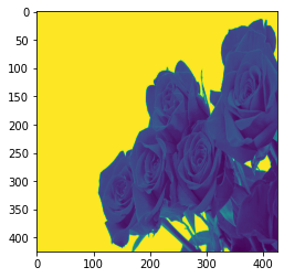
# create a mask of flag

lv = np.array([0, 0, 0])
hv = np.array([220, 220, 255])

mask = cv2.inRange(fg, lv, hv)
plt.imshow(mask)
plt.show()

masked_img = rgb_fg.copy()
masked_img[mask != 255] = [0, 0, 0]
plt.imshow(masked_img)
plt.show()

bg_cpy = rgb_pyramid.copy()
bg_cpy[mask == 255] = [0, 0, 0]

plt.imshow(bg_cpy)
plt.show()

final = bg_cpy + masked_img
plt.imshow(final)
plt.show()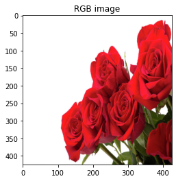

(2104, 3157, 3)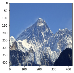

Exercise

• Use image with different background color for masking

High pass vs low pass filters

• Highpass are for sharpening image, enhance features and finding edges.
• Filters are convolutional kernels, ex [[0 -1 0] [-1 4 -1] [0 -1 0]]. Finds change between current and neighbor pixels.
• If output of convolution is 0 then no change if its -ve then its darken else brighter.
• For horizontal use ex [[-1 2 -1] [0 0 0] [-1 2 -1]].

# lets make a show function

def show(img, t = 'image', cmap='gray'):
    fig = plt.figure(figsize=(20,20))
    ax = fig.add_subplot(111)
    ax.imshow(img,cmap)
    plt.title(t)
    plt.show()

stripes = cv2.imread('(https://q-viper.github.io/assets/intro_opencv/coin.png', 0)
show(stripes)

# Sobel x
kernel1 = np.array([[ -1, 0, 1],
                 [ -2, 0, 2],
                 [ -1, 0, 1]])

filtered = cv2.filter2D(stripes, -1, kernel1)
show(filtered, 'Sobel_x')

# Sobel y
kernel2 = np.array([[ -1, -2, -1],
                 [ 0, 0, 0],
                 [ 1, 2, 1]])

filtered = cv2.filter2D(stripes, -1, kernel2)
show(filtered, 'Sobel_y')

kernel = kernel1 + kernel2

filtered = cv2.filter2D(stripes, -1, kernel)
show(filtered, 'Sobel')

Exercise

• Use different filters of highpass/lowpass

Low-pass Filters

• Blurring of image smoothen the image.
• We use low-pass filters for that.
• Low pass filters are mean filters, median filters weighted mean filters gaussian blur etc.
• Median blur removes salt and pepper noise.
• Averaging by: cv2.blur(img, depth, kernel) or cv2.boxFilter(img, depth, kernel, normalize..)
• Gaussian blur by: cv2.GaussainBlur(img, kernel, depth), cv2.getGaussianKernel(size, sigmax, sigmay)
• Median blur:cv2.medianBlur(img, 4) removes 40% of salt and pepper noise.

noise = cv2.imread('(https://q-viper.github.io/assets/intro_opencv/noise.png', 0)
show(noise)
kernel = np.ones([7, 7], dtype = np.float32)/255
blurred = cv2.filter2D(noise, -1, kernel)
show(blurred)

blurred = cv2.blur(noise, (5, 5))
show(blurred)

blurred = cv2.GaussianBlur(noise, (5, 5), -1)
show(blurred)

blurred = cv2.medianBlur(noise, 9)
show(blurred)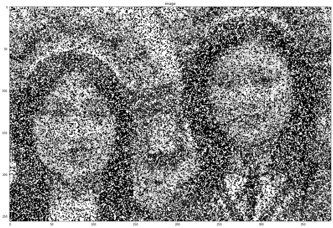

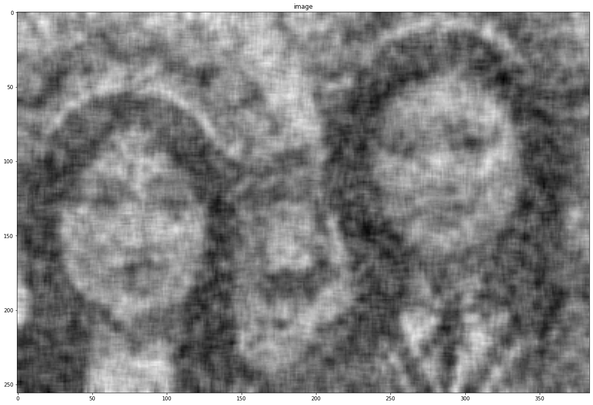
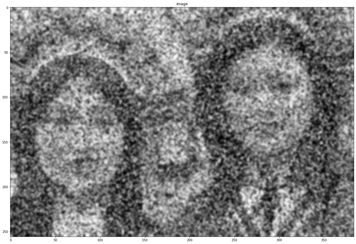
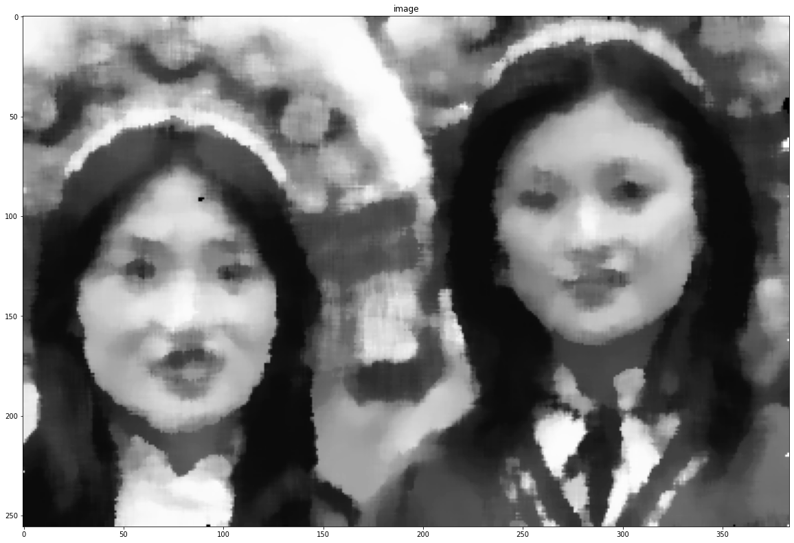
Image Thresholding

# Threshold
retval, thresholded = cv2.threshold(filtered, 100, 200, cv2.THRESH_BINARY)
show(thresholded)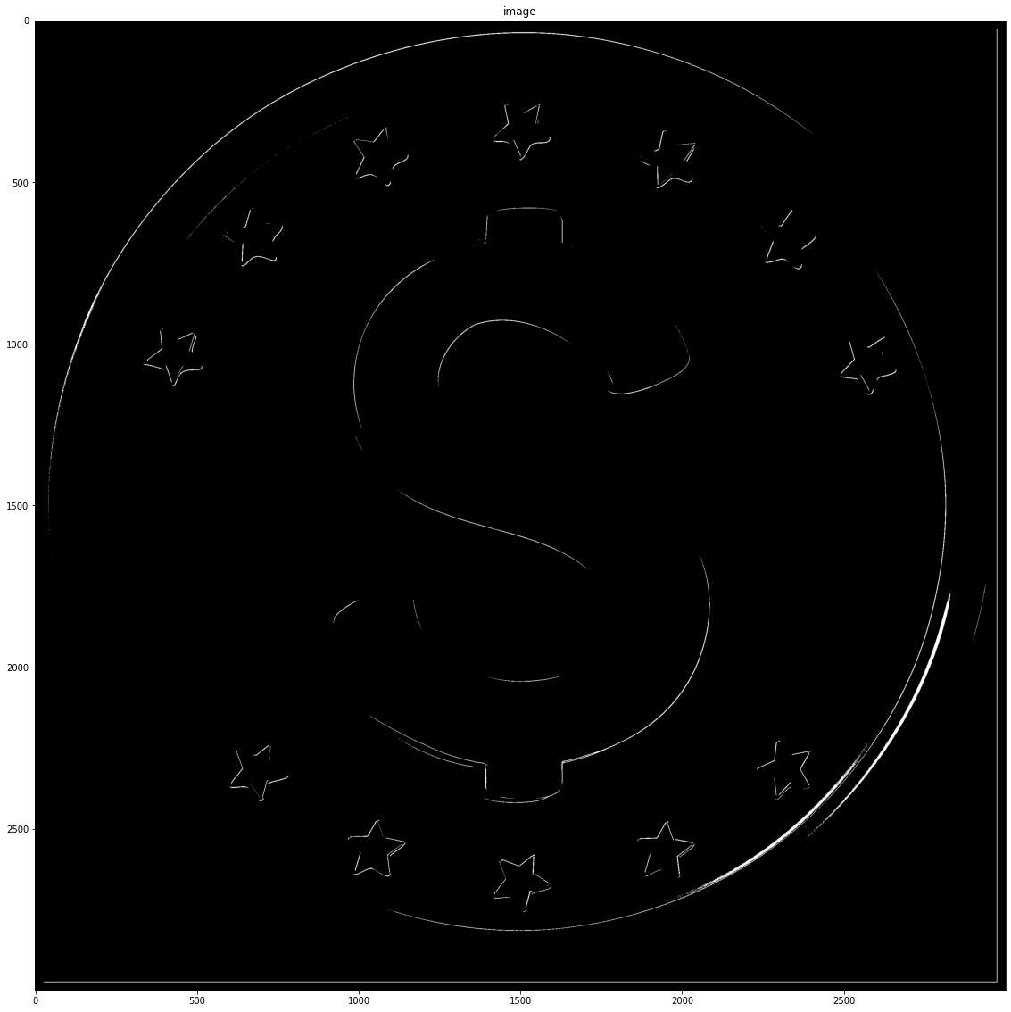

Exercise

• Use different blurring filters
• Use differnt kernels for filtering

Canny edge detector

Combination of processes:

• Noise filteration using Gaussian Blur
• Then Sobel filters
• Uses NMS for isolate strongest edges
• Hysteresis thresholding for best edges

# parameters

low = 10
high = 250

canny_img = cv2.Canny(stripes, low, high)

show(canny_img, "Canny")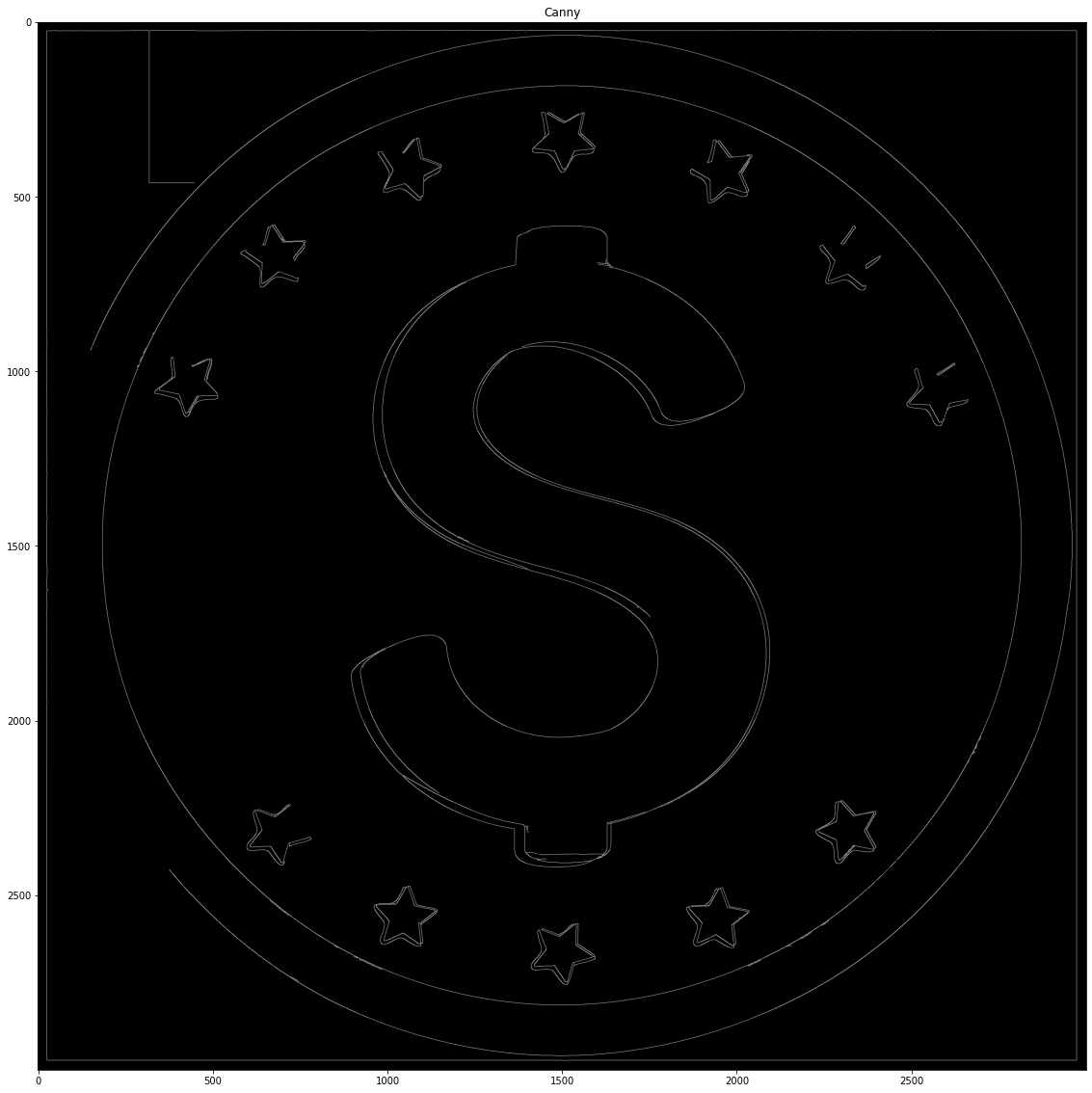

# Hough transform
img = cv2.imread('(https://q-viper.github.io/assets/intro_opencv/flag.jpg', 0)
show(img)

canny_img = cv2.Canny(img, low, high)
show(canny_img)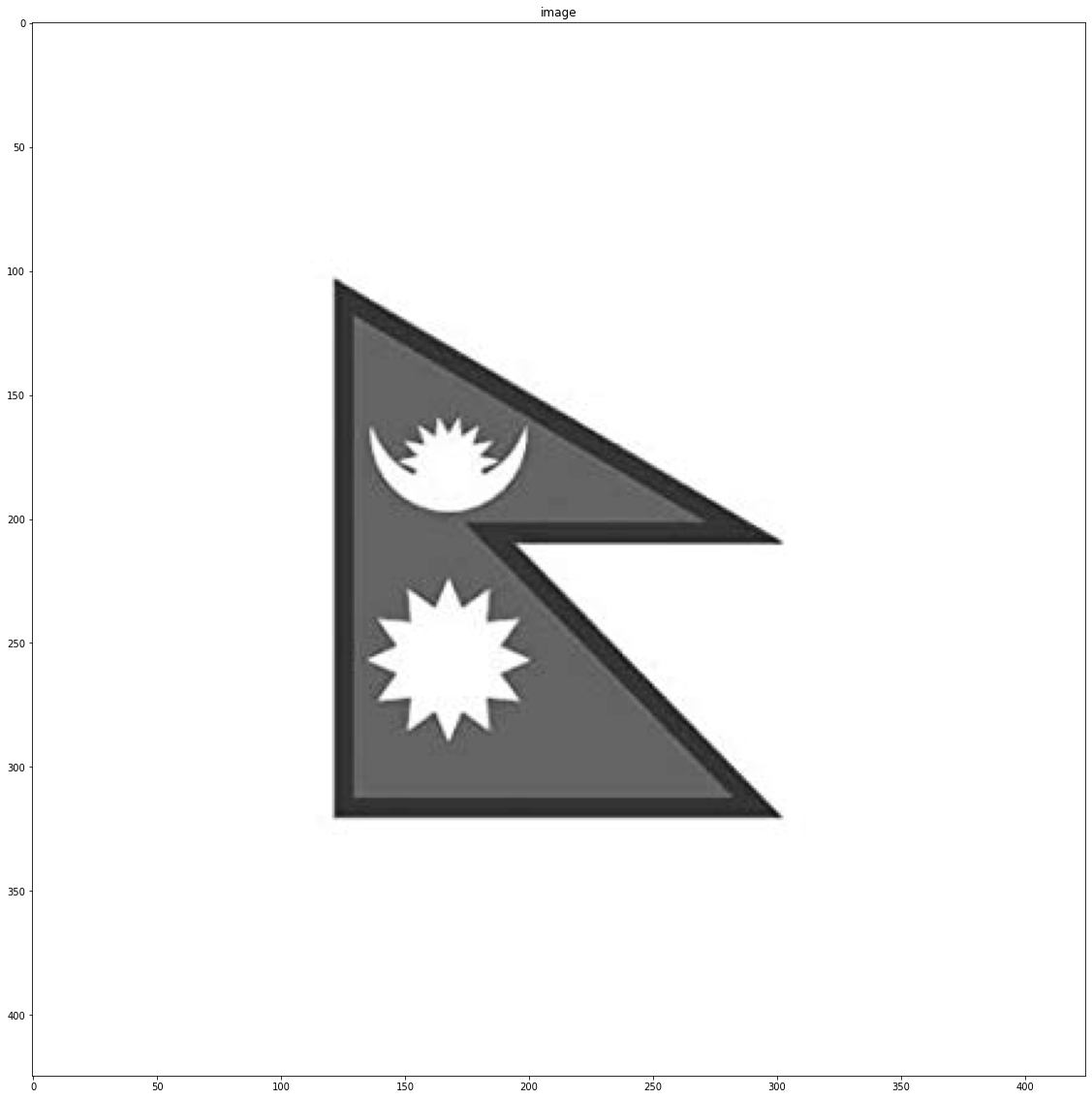

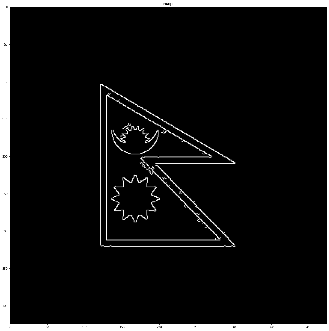
Hough Transform for line detection

#parameters
rho = 1
theta = np.pi / 180
threshold = 60
max_line_length = 50
max_line_gap = 50

lines = cv2.HoughLinesP(canny_img, rho, theta, threshold, np.array([]), max_line_length, max_line_gap)

line_img = img.copy()
for line in lines:
    for x1, y1, x2, y2 in line:
        cv2.line(line_img, (x1, y1), (x2, y2), (0, 255, 0), 2)

show(line_img)

Haar-cascades

# Haar Cascade
img = cv2.imread("(https://q-viper.github.io/assets/intro_opencv/xmen.jpg", 1)
gray = cv2.cvtColor(img, cv2.COLOR_BGR2GRAY)

# locate XML Haar Cascade file(it will be inside site packages/cv2/data)
cascade_dir = "C:\ProgramData\Anaconda3\Lib\site-packages\cv2\data/"

# face_cascade 
face_cascade = cv2.CascadeClassifier(cascade_dir + 'haarcascade_frontalface_default.xml')

# eye_cascade
eye_cascade = cv2.CascadeClassifier(cascade_dir + 'haarcascade_eye.xml')

# find bounding box coordinates of faces
faces = face_cascade.detectMultiScale(gray, 1.3, 5)
d=100
shape = gray.shape
# loop through each faces and draw a rectangle
for (x,y,w,h) in faces:
    y = np.clip(y-d, 0, y)
    x = np.clip(x-d, 0, x)
    w = np.clip(w+2*d, 0, shape[0]-x)
    h = np.clip(h+2*d, 0, shape[1]-y)
    img = cv2.rectangle(img,(x,y),(x+w,y+h),(255,0,0),2)
    roi_gray = gray[y:y+h, x:x+w]
    roi_color = img[y:y+h, x:x+w]
#     eyes = eye_cascade.detectMultiScale(roi_gray)

#     for (ex,ey,ew,eh) in eyes:
#         cv2.rectangle(roi_color,(ex,ey),(ex+ew,ey+eh),(0,255,0),2)

show(cv2.cvtColor(img, cv2.COLOR_BGR2RGBA))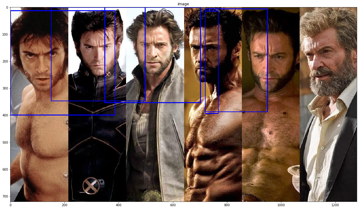

Exercise

• Use different haarcascades

Contours in OpenCv

Contours are simple curves that are joined around a object of same color or intensity. For example if we want to extract a edges of bottle, the contour curve will be around the bottle edges only. On OpenCv, contour can be drawn easily extracted and drawn.

img = cv2.imread('(https://q-viper.github.io/assets/intro_opencv/flag.jpg')
img_gray = cv2.cvtColor(img,cv2.COLOR_BGR2GRAY)

_, thresh = cv2.threshold(img_gray, 0, 255, cv2.THRESH_BINARY+cv2.THRESH_OTSU)
# show(thresh)

# ret, thresh = cv2.threshold(img_gray, 127, 255,0)
contours,hierarchy = cv2.findContours(thresh,2,1) # Gives contours points

cnt = contours[0]

# find the convex hull
hull = cv2.convexHull(cnt,returnPoints = False)

defects = cv2.convexityDefects(cnt,hull)

for i in range(defects.shape[0]):
    s,e,f,d = defects[i,0]
    start = tuple(cnt[s][0])
    end = tuple(cnt[e][0])
    far = tuple(cnt[f][0])
    cv2.line(img,start,end,[0,255,0],2)
    cv2.circle(img,far,5,[0,0,255],-1)

show(img)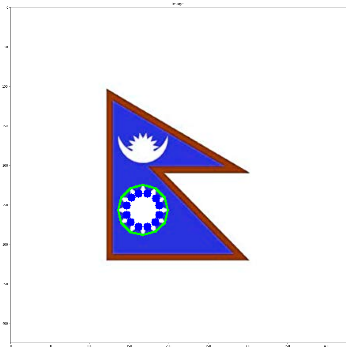

Color tracking on OpenCv

Using HSV colorspace, we can track any object very easily. HSV stands for Hue, S for Saturation and V for Value. Hue range is [0,179], Saturation range is [0,255] and Value range is [0,255]. Lets track white.

# Open Camera
cap = cv2.VideoCapture(0)

# While camera is on
while(1):

    # Take each frame
    _, frame = cap.read()

    # Convert BGR to HSV
    hsv = cv2.cvtColor(frame, cv2.COLOR_BGR2HSV)

    # take lower and upper white color range
    lower_white = np.array([0,0, 0], dtype=np.uint8)
    upper_white = np.array([20,20,255], dtype=np.uint8)

    # Threshold the HSV image to get only white colors
    mask = cv2.inRange(hsv, lower_white, upper_white)

    # Bitwise-AND mask and original image
    res = cv2.bitwise_and(frame,frame, mask= mask)

    cv2.imshow('frame',frame)
    cv2.imshow('mask',mask)
    cv2.imshow('res',res)
    k = cv2.waitKey(5) & 0xFF
    if k == 27:
        break

cap.release()
cv2.destroyAllWindows()