Lets write a Convolutional Neural Networks From Scratch. Writing Convoluitional Nerual Networks from Scratch is one of the challenging thing to be even for experienced person because we have been using frameworks like PyTorch to train and slowly forgetting basics of it.

What will you do when you are stuck in a village with no electricity for 4 days and you only have a pen and paper? For me, I wrote a Convolutional Neural Networks from Scratch on paper. Once again, high credit goes to the pandemic Corona Virus, without it, I would not have lived as a farmer once more and the idea of ' from scratch' arose.

I am sorry for not using a single image here on this blog because I was low on data and this entire blog is written on markdown(sometimes latex) only so the text format might seem a little disturbing also.

If you are here, then you are encouraged to look at the below 3 blog posts(serially) of mine(most of the concepts on this blog are taken from the below posts):

• Writing a Feedforward Neural Network from Scratch on Python
  • This post gives a brief introduction to an OOP concept of making a simple Keras-like ML library.
  • A gentle introduction to backpropagation and gradient descent from scratch.
• Writing top Machine Learning Optimizers from scratch on Python
  • Gives introduction and python code to optimizers like GradientDescent and ADAM`.
• Writing a Image Processing Codes from Scratch on Python
  • This post gives a brief introduction to convolution operation and RGB to grayscale conversion from scratch.
  • We will be using the same convolution concept here on this blog.

If you are less on time then follow this repository for all the files, also see inside the folder quark.

Updates:

• 2020/06/05: Published blog.
• 2022/11/10: Fixed errors in the derivative.

1.1 What this Convolutional Neural Networks from Scratch blog will cover?

• Includes Feed forward layer
• A gentle introduction to Conv2d
• Includes Dropout layer
• Includes Pool2d layer
• Includes Flatten layer
• Test Cases with different architectures(4 of them) on MNIST dataset
• Bonus Topics

Testing a model will require huge time, my system is Dell I5 with 8GB RAM and 256GB SSD. And I tested these models on my local machine. It had taken nearly a week to find the test cases and improve the overall concepts. Sometimes, I had to sleep on my laptop for saving battery power so some epochs might be seen taking 4+hours of time. And yes, I used mobile data to post this blog.

2 Preliminary Concepts for Convolutional Neural Networks from Scratch

• Every layer will have the common methods(doing so will ease the overhead of method calling):
  • set_output_shape
  • apply_activation
    • Conv2d can have functions like relu and convolution operation happens here
    • FFL will use the activation_fn method on a linear combination of input, weights, and biases.
    • Pool2d will perform pooling operations like max, min, average
    • Dropout will perform setting input to 0 randomly
    • Flatten will convert feature vectores to 1d vector
  • backpropagate
    • Conv2d will use the delta term of the next layer to find the delta term and delta parameters
    • FFL
    • Pool2d: error is backpropagated from the index of the output of this layer
    • Dropout: propagate error through non-zero output units
    • Flatten: propagate error of next layer to previous by reshaping to input shape

3 Steps

• Prepare layers
• Prepare stacking class
• Prepare Optimizers

3.1 Prepare Layers

Let's prepare layers from scratch for Convolutional Neural Networks from Scratch.

3.1.1 Feedforward Layer

For a typical Convolutional Neural Networks from Scratch, we need a feedforward layer as well. I am not going to explain much more here because a previous post about Writing a Feedforward Neural Network from Scratch on Python has explained already.

   class FFL():
    def __init__(self, input_shape=None, neurons=1, bias=None, weights=None, activation=None, is_bias = True):
        np.random.seed(100)
        self.input_shape = input_shape
        self.neurons = neurons
        self.isbias = is_bias
        self.name = ""
        self.w = weights
        self.b = bias
        if input_shape != None:
            self.output_shape = neurons                
        if self.input_shape != None:
            self.weights = weights if weights != None else np.random.randn(self.input_shape, neurons)
            self.parameters = self.input_shape *  self.neurons + self.neurons if self.isbias else 0  
        if(is_bias):
            self.biases = bias if bias != None else np.random.randn(neurons)
        else:
            self.biases = 0            
        self.out = None
        self.input = None
        self.error = None
        self.delta = None
        activations = ["relu", "sigmoid", "tanh", "softmax"]
        self.delta_weights = 0
        self.delta_biases = 0
        self.pdelta_weights = 0
        self.pdelta_biases = 0        
        if activation not in activations and activation != None:
             raise ValueError(f"Activation function not recognised. Use one of {activations} instead.")
        else:
            self.activation = activation   

    def activation_dfn(self, r):
        """
            A method of FFL to find the derivative of a given activation function.
        """     
        if self.activation is None:
            return np.ones(r.shape)
        if self.activation == 'tanh':
            return 1 - r ** 2
        if self.activation == 'sigmoid':
            # r = self.activation_fn(r)
            return r * (1 - r)
        if self.activation == "softmax":
            soft = self.activation_fn(r)                                
            diag_soft = soft*(1- soft)
            return diag_soft  
        if self.activation == 'relu':
            r[r < 0] = 0
            r[r>=1]=1
            return r
        return r

    def activation_fn(self, r):
        """
        A method of FFL that contains the operation and definition of a given activation function.
        """        
        if self.activation == 'relu':
            r[r < 0] = 0
            return r
        if self.activation == None or self.activation == "linear":
            return r        
        if self.activation == 'tanh':
            return np.tanh(r)
        if self.activation == 'sigmoid':    
            return 1 / (1 + np.exp(-r))
        if self.activation == "softmax":
            r = r - np.max(r)
            s = np.exp(r)
            return s / np.sum(s)        
    def apply_activation(self, x):
        soma = np.dot(x, self.weights) + self.biases
        self.out = self.activation_fn(soma)        
        return self.out

    def set_n_input(self):
        self.weights = self.w if self.w != None else np.random.normal(size=(self.input_shape, self.neurons))

    def backpropagate(self, nx_layer):
        self.error = np.dot(nx_layer.weights, nx_layer.delta)
        self.delta = self.error * self.activation_dfn(self.out)
        self.delta_weights += self.delta * np.atleast_2d(self.input).T
        self.delta_biases += self.delta

    def set_output_shape(self):
        self.set_n_input()
        self.output_shape = self.neurons
        self.get_parameters()

    def get_parameters(self):
        self.parameters = self.input_shape *  self.neurons + self.neurons if self.isbias else 0  
        return self.parameters 

3.1.2 Conv2d Layer

This layer will be the crucial layer for Convolutional Neural Networks from Scratch.

3.1.2.1 Let's initialize it first.

class Conv2d():
    def __init__(self, input_shape=None, filters=1, kernel_size = (3, 3), isbias=True, activation=None, stride=(1, 1),             padding="zero", kernel=None, bias=None):
        self.input_shape = input_shape
        self.filters = filters
        self.isbias = isbias
        self.activation = activation
        self.stride = stride
        self.padding = padding
        self.p = 1 if padding != None else 0
        self.bias = bias
        self.kernel = kernel
        if input_shape != None:
            self.kernel_size = (kernel_size[0], kernel_size[1], input_shape[2], filters)
            self.output_shape = (int((input_shape[0] - kernel_size[0] + 2 * self.p) / stride[0]) + 1, 
                                int((input_shape[1] - kernel_size[1] + 2 * self.p) / stride[1]) + 1, filters)
            self.set_variables()
            self.out = np.zeros(self.output_shape)
        else:
            self.kernel_size = (kernel_size[0], kernel_size[1])         

Initializing takes:-

• input_shape:- It is the input shape of this layer. It will include a tuple of (rows, cols, num_channels). For any noninput layer, it will default i.e. None.
• filters:- How many kernels or filters are we using?
• kernel_size:- It is the size of convoluting tuple of matrix or filter's (row, cols). Later we will create a kernel of shape rows, cols, input_channels, num_filters.
• isbias: Boolean value for whether we will use bias or not.
• activaiton: Activation function.
• tride: A tuple indicating a step of convolution operation per row, column.
• padding: String indicating what operation will be done on borders, available among [zeros, same].
• kernel: A convoluting matrix. Recommended not to use it.
• bias: A array of shape (num_filters, 1) will be added after each convolution operation.

A few important things inside this method are:-

• The output_shape of any convolution layer will be: \begin{equation} W = \frac{(w-f+2*p)}{s} + 1 \end{equation}

  Where W is output width or shape and w is input width or shape.\ f is filter width.\ p is padding(1 if used)\ s is stride width or shape\

• The method set_variables() sets all the important parameters needed for training.
• self.out will be the output of this layer and self.dout will be the delta out.
• self.delta will be the delta term of this layer

3.1.2.2 set_variable() method

def set_variables(self):
    self.weights = self.init_param(self.kernel_size)
    self.biases = self.init_param((self.filters, 1))
    self.parameters = np.multiply.reduce(self.kernel_size) + self.filters if self.isbias else 1
    self.delta_weights = np.zeros(self.kernel_size)
    self.delta_biases = np.zeros(self.biases.shape)    

• To make our optimization easier, we are naming filters as weights.
• The method init_param() initializes the parameter from the random normal sample.

def init_param(self, size):
    stddev = 1/np.sqrt(np.prod(size))
    return np.random.normal(loc=0, scale=stddev, size=size)

3.1.2.3 Prepare Activation Functions

def activation_fn(self, r):
    """
    A method of FFL that contains the operation and definition of a given activation function.
    """
    if self.activation == None or self.activation == "linear":
        return r   
    if self.activation == 'tanh': #tanh
        return np.tanh(r)
    if self.activation == 'sigmoid':  # sigmoid
        return 1 / (1 + np.exp(-r))
    if self.activation == "softmax":# stable softmax   
        r = r - np.max(r)
        s = np.exp(r)
        return s / np.sum(s)

Recall the mathematics,

\begin{equation} i. tanh(soma) = \frac{1-soma}{1+soma} \end{equation}

\begin{equation} ii. linear(soma) = soma \end{equation}

\begin{equation} iii. sigmoid(soma) = \frac{1}{1 + exp^{(-soma)}} \end{equation}

\begin{equation} iv. relu(soma) = \max(0, soma) \end{equation}

\begin{equation} v. softmax(x_j) = \frac{exp^{(xj)}}{\sum{i=1}^n{exp^{(x_i)}}} \end{equation}

\begin{equation} Where, soma = XW + \theta \end{equation}

And W is the weight vector of shape (n, w). X is the input vector of shape (m, n) and 𝜃 is the bias term of shape w, 1.

3.1.2.4 Prepare derivative of Activation Function

def activation_dfn(self, r):
        """
            A method of FFL to find the derivative of a given activation function.
        """
        if self.activation is None:
            return np.ones(r.shape)
        if self.activation == 'tanh':
            return 1 - r ** 2
        if self.activation == 'sigmoid':
            return r * (1 - r)
        if self.activtion == 'softmax':
            soft = self.activation_fn(r)
            return soft * (1 - soft)
        if self.activation == 'relu':
            r[r<0] = 0
            r[>=1]=1
            return r

Let's revise a bit of calculus.

Why do we need derivative?

While doing Convolutional Neural Networks from Scratch, we need to do few derivatives. Well, if you are here then you already know that gradient descent is based on the derivatives(gradients) of activation functions and errors. So we need to perform this derivative. But you are on your own to perform calculations. I will also explain the gradient descent later.

\begin{equation} i. \frac{d(linear(x))}{d(x)} = 1 \end{equation}

\begin{equation} ii. \frac{d(sigmoid(x))}{d(x)} = sigmoid(x)(1- sigmoid(x)) \end{equation}

\begin{equation} iii. \frac{d(tanh(x))}{d(x)} = 1-tanh(x)**2 \end{equation}

\begin{equation} iv. \frac{d(relu(x))}{d(x)} = 1 if x>=1 else 0 \end{equation}

\begin{equation} v. \frac{d(softmax(x_j))}{d(x_k)} = softmax(x_j)(1- softmax(x_j)) \space when \space j = k \space else\ \space -softmax({x_j}).softmax({x_k}) \end{equation}

For the sake of simplicity, we use the case of j = k for softmax.

3.1.2.5 Prepare a method to do feedforward on this layer

    def apply_activation(self, image):
        for f in range(self.filters):
            image = self.input
            kshape = self.kernel_size
            if kshape[0] % 2 != 1 or kshape[1] % 2 != 1:
                raise ValueError("Please provide odd length of 2d kernel.")
            if type(self.stride) == int:
                     stride = (stride, stride)
            else:
                stride = self.stride
            shape = image.shape
            if self.padding == "zero":
                zeros_h = np.zeros((shape[1], shape[2])).reshape(-1, shape[1], shape[2])
                zeros_v = np.zeros((shape[0]+2, shape[2])).reshape(shape[0]+2, -1, shape[2])
                padded_img = np.vstack((zeros_h, image, zeros_h)) # add rows
                padded_img = np.hstack((zeros_v, padded_img, zeros_v)) # add cols
                image = padded_img
                shape = image.shape
            elif self.padding == "same":
                h1 = image[0].reshape(-1, shape[1], shape[2])
                h2 = image[-1].reshape(-1, shape[1], shape[2])
                padded_img = np.vstack((h1, image, h2)) # add rows
                v1 = padded_img[:, 0].reshape(padded_img.shape[0], -1, shape[2])
                v2 = padded_img[:, -1].reshape(padded_img.shape[0], -1, shape[2])
                padded_img = np.hstack((v1, padded_img, v2)) # add cols
                image = padded_img
                shape = image.shape
            elif self.padding == None:
                pass
            rv = 0
            cimg = []
            for r in range(kshape[0], shape[0]+1, stride[0]):
                cv = 0
                for c in range(kshape[1], shape[1]+1, stride[1]):
                    chunk = image[rv:r, cv:c]
                    soma = (np.multiply(chunk, self.weights[:, :, :, f]))
                    summa = soma.sum()+self.biases[f]
                    cimg.append(summa)
                    cv+=stride[1]
                rv+=stride[0]
            cimg = np.array(cimg).reshape(int(rv/stride[0]), int(cv/stride[1]))
            self.out[:, :, f] = cimg
        self.out = self.activation_fn(self.out)
        return self.out

I have linked a post about convolution operation at the top of this blog. The only important part here is:-

• For each filter
  • do elementwise matrix multiplication and sum them all(of each channels also)
  • Then add bias term
  • Output of this filter will have channel(not a real color channel) of num_filters
• Finally apply the activation function on this output.

It is clear that, if a layer has 5 filters then the output of this layer will have 5 channels also.

3.1.2.6 Prepare Method for Backpropagation

    def backpropagate(self, nx_layer):
        layer = self
        layer.delta = np.zeros((layer.input_shape[0], layer.input_shape[1], layer.input_shape[2]))
        image = layer.input
        for f in range(layer.filters):
            kshape = layer.kernel_size
            shape = layer.input_shape
            stride = layer.stride
            rv = 0
            i = 0
            for r in range(kshape[0], shape[0]+1, stride[0]):
                cv = 0
                j = 0
                for c in range(kshape[1], shape[1]+1, stride[1]):
                    chunk = image[rv:r, cv:c]
                    layer.delta_weights[:, :, :, f] += chunk * nx_layer.delta[i, j, f]
                    layer.delta[rv:r, cv:c, :] += nx_layer.delta[i, j, f] * layer.weights[:, :, :, f]
                    j+=1
                    cv+=stride[1]
                rv+=stride[0]
                i+=1
            layer.delta_biases[f] = np.sum(nx_layer.delta[:, :, f])
        layer.delta = layer.activation_dfn(layer.delta)

Backpropagating error from the Convolution layer is a really hard and challenging task. I have tried my best to do the right way of backpropagation but I still have doubt about it. Some really awesome articles like below can help to understand these things:-

• Convolutional Neural Network from Ground Up
• A Gentle Introduction to CNN
• Training a Convolutional Neural Networks from Scratch

For understanding how to pass errors and find the delta terms for parameters:

• The delta term for this layer will be equal to the shape of the input i.e. (input_row, input_cols, input_channels).
• We will also take the input to this layer into consideration.
• For each filter:-
  • Loop through each row and col just like the convolution operation
  • Get the chunk or part of the image and multiply it with the delta term of the next layer to get the delta filter(weight)
    • i.e. layer.delta_weights[:, :, :, f] += chunk * nx_layer.delta[i, j, f] a trick to understanding the delta of the next layer is by revisiting the input and output shape of the layer. For a layer with 5 filters, the output will have 5 channels. And the delta term of the next layer will have the same number of channels. Hence we are giving [i, j, f]. Note that for every step on the input image(i.e step on row and col), i, j will increase by 1. Initially, layer.delta_weights[:, :, :, f] will be all 0s but it will change by visiting every chunk. Since we have a filter of shape (row, col, channels, num_filters), delta_weights is updated for each filter by adding it with the multiplication of each chunk with the corresponding next layer's delta.
    • Delta term of this layer will have shape of (input_rows, input_cols, channels) i.e equal to input shape. Hence we will set the delta term using the number of channels on this layer's filters. We will add the delta term for that chunk using each filter. Because each filter is responsible for the error and the contribution of each filter must be taken equally. The layer.delta[rv:r, cv:c, :] += nx_layer.delta[i, j, f] * layer.weights[:, :, :, f] is here to do this task.
    • We increase I after completing the row and j after completing the column. i and j are used to getting values from the delta of the next layer.
  • We sum the delta term of this filter to get delta_biases due to this filter.
• Finally, we get the delta of this layer by applying the derivative of the activation function of this layer.

There are different approaches than this one of doing backpropagation on the Convolution layer. I found this one to be working on my case(i wrote this approach). Please try to visit one of the above links for more explanation.

Please test your class like below:-

img = xt[0]
conv = Conv2d()
conv.input=img
conv.weights = np.array([[1, 0, -1], [1, 0, -1], [1, 0, -1]]).reshape(3, 3, 1, 1)
conv.biases = np.zeros(1)
conv.out = np.zeros((28, 28, 1))
cout = conv.apply_activation(img)
plt.imshow(cout.reshape(28, 28)) 

Where xt is an image array of shape (28, 28, 1) from mnist.

3.1.3 Dropout Layer

The main concept behind the dropout layer is to forget some of the inputs to the current layer forcefully. Doing so will reduce the risk of overfitting the model.

class Dropout:
    def __init__(self, prob = 0.5):
        self.input_shape=None
        self.output_shape = None
        self.input_data= None
        self.output = None
        self.isbias = False
        self.activation = None
        self.parameters = 0
        self.delta = 0
        self.weights = 0
        self.bias = 0
        self.prob = prob
        self.delta_weights = 0
        self.delta_biases = 0       
    def set_output_shape(self):
        self.output_shape = self.input_shape
        self.weights = 0
    def apply_activation(self, x, train=True):
        if train:
            self.input_data = x
            flat = np.array(self.input_data).flatten()
            random_indices = np.random.randint(0, len(flat), int(self.prob * len(flat)))
            flat[random_indices] = 0
            self.output = flat.reshape(x.shape)
            return self.output
        else:
            self.input_data = x
            self.output = x / self.prob
            return self.output
    def activation_dfn(self, x):
        return x
    def backpropagate(self, nx_layer):
        if type(nx_layer).__name__ != "Conv2d":
            self.error = np.dot(nx_layer.weights, nx_layer.delta)
            self.delta = self.error * self.activation_dfn(self.out)
        else:
            self.delta = nx_layer.delta
        self.delta[self.output == 0] = 0

• Some of the parameters like weights, biases are actually not available on the Dropout layer but I am using this for the sake of simplicity while working with a stack of layers.
• The input shape and output shape of the Dropout layer will be the same, what differs is the value. Where some will be set to 0 i.e forgotten randomly.
• The method apply_activation performs the dropout operation.
  • The easier way is to first convert it to a 1d vector(by NumPy's flatten) and take random indices from a given probability.
  • Then we set the element of those random indices to 0 and return the reshaped new array as the output of this layer.
• The method backpropagate performs the backpropagation operation on error.
  • We set the delta to 0 if the recent output of this layer is 0, else leave it as it is.
• Note:- In the testing phase, forward propagation will be different. Entire activation is reduced by a factor. So we are also giving a training parameter to apply_activation.

Lets test our class:-

x = np.arange(0, 100).reshape(10, 10)
dp = Dropout()
dp.apply_activation(x)

3.1.4 Pooling Layer

A convolutional neural network's work can be thought of as:

• Take an image where we want to perform a convolution.
• Take a lens(will be filtered) and place it over an image.
• Slide the lens over an image and find the important features.
• We find features using different lenses.
• Once we found certain features under our boundary, we pass those feature maps to the next scanning place or we can do pooling.
• Pooling can be thought of as zooming out, or we make the remaining image a little smaller, by this way more important features will be seen. Or in another way, scan from a bit far and take only the important parts.

A pooling operation works in a similar way to convolution but instead of matrix multiplication, we do a different operation. The output of a pooling layer will be:-

\begin{equation} w = \frac{W-f + 2p}{s} + 1 \end{equation}

where w is the new width, W is the old or input width, f is kernel width, p is padding. I am not using padding right now for the operation.

3.1.4.1 Initializing a Class

class Pool2d:
    def __init__(self, kernel_size = (2, 2), stride=None, kind="max", padding=None):
        self.input_shape=None
        self.output_shape = None
        self.input_data= None
        self.output = None
        self.isbias = False
        self.activation = None
        self.parameters = 0
        self.delta = 0
        self.weights = 0
        self.bias = 0
        self.delta_weights = 0
        self.delta_biases = 0
        self.padding = padding
        self.p = 1 if padding != None else 0
        self.kernel_size = kernel_size
        if type(stride) == int:
                 stride = (stride, stride)
        self.stride = stride
        if self.stride == None:
            self.stride = self.kernel_size
        self.pools = ['max', "average", 'min']
        if kind not in self.pools:
            raise ValueError("Pool kind not understood.")            
        self.kind = kind

Most of the attributes are common to the `Convolution layer.

• Just like Keras, we will set the stride to kernel_size if nothing is given.
• The pool is a list of available pooling types. Currently, I have only included 3.

3.1.4.2 Method set_output_shape

As always, this method will always be called from the stacking class.

    def set_output_shape(self):
        self.output_shape = (int((self.input_shape[0] - self.kernel_size[0] + 2 * self.p) / self.stride[0] + 1), 
                            int((self.input_shape[1] - self.kernel_size[1] + 2 * self.p) / self.stride[1] + 1),                                         self.input_shape[2])       

3.1.4.3 Feedforward or apply_activation method

This method will perform the real pooling operation indicated above.

    def apply_activation(self, image):
        stride = self.stride
        kshape = self.kernel_size
        shape = image.shape
        self.input_shape = shape
        self.set_output_shape()
        self.out = np.zeros((self.output_shape))
        for nc in range(shape[2]):
            cimg = []
            rv = 0
            for r in range(kshape[0], shape[0]+1, stride[0]):
                cv = 0
                for c in range(kshape[1], shape[1]+1, stride[1]):
                    chunk = image[rv:r, cv:c, nc]
                    if len(chunk) > 0:                        
                        if self.kind == "max":
                            chunk = np.max(chunk)
                        if self.kind == "min":
                            chunk = np.min(chunk)
                        if self.kind == "average":
                            chunk = np.mean(chunk)
                        cimg.append(chunk)
                    else:
                        cv-=cstep
                    cv+=stride[1]
                rv+=stride[0]
            cimg = np.array(cimg).reshape(int(rv/stride[0]), int(cv/stride[1]))
            self.out[:,:,nc] = cimg
        return self.out

Lets take an example:-

$$

\begin{equation} x = \begin{pmatrix} 1 & 2 & 3 & 1 \\ 11 & 12 & 4 & 10 \\ 101 & 11 & 88 & 10 \\ 10 & 11 & 11 & 5 \end{pmatrix} \end{equation}

$$

After maxpool of size (2, 2) and stride (2, 2):-

• First our pointer will be 0 for row/col i.e curr_pointer = (0, 0) and window will be values of curr_pointer:curr_pointer+kernel_size-1.
• In other words, our first window will be [[1 2] [11, 12]].
• Then for the max pool, the maximum value on this window is 12, so 12 is taken, if the average pool then the output of this window will be 6.5 i.e average of 1, 2, 11, 12.
• Then current pointer of row will be prev_pointer[0]+stride[0]
• Now the new window will be [[3 1] [4 10]] and the max pool will be 10.
• Now we have reached the end of this row, we will increase the column. Then the current pointer will be curr_pointer + (0, stride[1]-1).

Maxpooling of 𝑥:

$$ \begin{pmatrix} 12 & 10 \\ 101 & 88 \end{pmatrix} $$

In a simpler way, we took only those values which contribute to high value.

3.1.4.4 Backpropagate Method

def backpropagate(self, nx_layer):
    """
        Gradients are passed through an index of the latest output value.
    """
    layer = self
    stride = layer.stride
    kshape = layer.kernel_size
    image = layer.input
    shape = image.shape
    layer.delta = np.zeros(shape)
    cimg = []
    rstep = stride[0]
    cstep = stride[1]
    for f in range(shape[2]):
        i = 0
        rv = 0
        for r in range(kshape[0], shape[0]+1, rstep):
            cv = 0
            j = 0
            for c in range(kshape[1], shape[1]+1, cstep):
                chunk = image[rv:r, cv:c, f]
                dout = nx_layer.delta[i, j, f]
                if layer.kind == "max":
                    p = np.max(chunk)
                    index = np.argwhere(chunk == p)[0]
                    layer.delta[rv+index[0], cv+index[1], f] = dout
                if layer.kind == "min":
                    p = np.min(chunk)
                    index = np.argwhere(chunk == p)[0]
                    layer.delta[rv+index[0], cv+index[1], f] = dout
                if layer.kind == "average":
                    p = np.mean(chunk)
                    layer.delta[rv:r, cv:c, f] = dout
                j+=1
                cv+=cstep
            rv+=rstep
            i+=1

The main idea behind the backpropagation on Pooling Layer is:-

• If pooling is Max then an error is passed through an index of the largest value on the chunk.
• If pooling is Minthen error is passed through an index of the smallest value on the chunk.
• If pooling is average then an error is passed through entire indices on a chunk

Since the output shape and input shape's number of the channel remain the same, we loop through each channel and get the delta for each channel. So we are not adding the delta term.

Lets test our pooling class:

pool = Pool2d(kernel_size=(7, 7), kind="max")
test = np.random.randint(1, 100, (32, 32, 3))
o = pool.apply_activation(test)

If you don't get any errors then, great let's proceed. Else please see the reference file on GitHub.

3.1.5 Flatten Layer

Flatten layer's main task is to take entire feature maps of the previous layer and make a 1d vector from it. Flatten layer is used before passing a result of convolution to classification layers.

Let the input to Flatten be (3, 3, 3).

$$ \begin{equation} x = \begin{pmatrix} \begin{pmatrix} 1 & 2 & 3\end{pmatrix} \begin{pmatrix} 1 & 11 & 12\end{pmatrix} \begin{pmatrix} 4 & 10 & 1\end{pmatrix}\\ \begin{pmatrix} 101 & 11 & 88\end{pmatrix} \begin{pmatrix} 10 & 11 & 11\end{pmatrix} \begin{pmatrix} 5 & 111 & 33\end{pmatrix}\\ \begin{pmatrix} 9 & 11 & 123\end{pmatrix} \begin{pmatrix} 66 & 110 & 12\end{pmatrix} \begin{pmatrix} 100 & 11 & 12\end{pmatrix} \end{pmatrix} \end{equation} $$

Flatten output will be:

$$ \begin{equation} \begin{pmatrix} 1 & 2 & 3& 1 & 11 & 12& 4 & 10 & 1& 101 & 11 & 88& 10 & 11 & 11& 5 & 111 & 33& 9 & 11 & 123& 66 & 110 & 12& 100 & 11 & 12& \end{pmatrix} \end{equation} $$

class Flatten:
    def __init__(self, input_shape=None):
        self.input_shape=None
        self.output_shape = None
        self.input_data= None
        self.output = None
        self.isbias = False
        self.activation = None
        self.parameters = 0
        self.delta = 0
        self.weights = 0
        self.bias = 0
        self.delta_weights = 0
        self.delta_biases = 0        
    def set_output_shape(self):
        self.output_shape = (self.input_shape[0] * self.input_shape[1] * self.input_shape[2])
        self.weights = 0
    def apply_activation(self, x):
        self.input_data = x
        self.output = np.array(self.input_data).flatten()
        return self.output
    def activation_dfn(self, x):
        return x
    def backpropagate(self, nx_layer):
        self.error = np.dot(nx_layer.weights, nx_layer.delta)
        self.delta = self.error * self.activation_dfn(self.out)
        self.delta = self.delta.reshape(self.input_shape)

Note: There will be no attributes like weights, biases on Flatten layer but I used to make it work on doing optimization

• The output shape of this layer will be the multiplication of (num_rows, num_cols, num_channels).
• Since this layer will be connected before the feedforward layer, error and delta terms are calculated like on the feedforward layer.
• The shape of the delta of this layer will be the shape of the input.

Lets test our flatten class:

x = np.array([[1, 1, 1], [1, 0, 1], [0, 1, 1], [0, 0, 1]])
f = Flatten()
print(f.apply_activation(test))  

If you got output like the below, then cool:-

[1, 1, 1, 1, 0, 1, 0, 1, 1, 0, 0, 1]

3.2 Creating a Stacking class

We will name it CNN.

As previous feedforward post, this will perform all the tasks like training, testing and so on.

3.2.1 Initializing a class

Please refer to the previous post about Feedforward Neural Networks for more explanation.

class CNN():
    def __init__(self):
        self.layers = []
        self.info_df = {}
        self.column = ["LName", "Input Shape", "Output Shape", "Activation", "Bias"]
        self.parameters = []
        self.optimizer = ""
        self.loss = "mse"
        self.lr = 0.01
        self.mr = 0.0001
        self.metrics = []
        self.av_optimizers = ["sgd", "momentum", "adam"]
        self.av_metrics = ["mse", "accuracy", "cse"]
        self.av_loss = ["mse", "cse"]
        self.iscompiled = False
        self.model_dict = None
        self.out = []
        self.eps = 1e-15
        self.train_loss = {}
        self.val_loss = {}
        self.train_acc = {}
        self.val_acc = {}    

3.2.2 Creating a add Method

Please refer to the previous post for more explanation.

def add(self, layer):
        if(len(self.layers) > 0):
            prev_layer = self.layers[-1]
            if prev_layer.name != "Input Layer":
                prev_layer.name = f"{type(prev_layer).__name__}{len(self.layers) - 1}"             
            if layer.input_shape == None:
                if type(layer).__name__ == "Flatten":
                        ops = prev_layer.output_shape[:]
                        if type(prev_layer).__name__ == "Pool2d":
                            ops = prev_layer.output_shape[:]
                elif type(layer).__name__ == "Conv2d":
                    ops = prev_layer.output_shape[:]
                    if type(prev_layer).__name__ == "Pool2d":
                        ops = prev_layer.output_shape
                elif type(layer).__name__ == "Pool2d":
                    ops = prev_layer.output_shape[:]
                    if type(prev_layer).__name__ == "Pool2d":
                        ops = prev_layer.output_shape[:]
                else:
                    ops = prev_layer.output_shape
                layer.input_shape = ops
                layer.set_output_shape()
            layer.name = f"Out Layer({type(layer).__name__})"
        else:
            layer.name = "Input Layer"
        if type(layer).__name__ == "Conv2d":
            if(layer.output_shape[0] <= 0 or layer.output_shape[1] <= 0):
                raise ValueError(f"The output shape became invalid [i.e. {layer.output_shape}]. Reduce filter size or increase image size.")
        self.layers.append(layer)
        self.parameters.append(layer.parameters)

3.2.3 Writing a summary method:

Please refer to the previous post for more explanation.

    def summary(self):
        lname = []
        linput = []
        loutput = []
        lactivation = []
        lisbias = []
        lparam = []
        for layer in self.layers:
            lname.append(layer.name)
            linput.append(layer.input_shape)
            loutput.append(layer.output_shape)
            lactivation.append(layer.activation)
            lisbias.append(layer.isbias)
            lparam.append(layer.parameters)
        model_dict = {"Layer Name": lname, "Input": linput, "Output Shape": loutput,
                      "Activation": lactivation, "Bias": lisbias, "Parameters": lparam}    
        model_df = pd.DataFrame(model_dict).set_index("Layer Name")
        print(model_df)
        print(f"Total Parameters: {sum(lparam)}")

Test the class:

m = CNN()
m.add(Conv2d(input_shape = (28, 28, 1), filters = 2, padding=None, kernel_size=(3, 3), activation="relu"))
m.add(Conv2d(filters=4, kernel_size=(3, 3), padding=None, activation="relu"))
m.add(Pool2d(kernel_size=(2, 2)))
m.add(Conv2d(filters=6, kernel_size=(3, 3), padding=None, activation="relu"))
m.add(Conv2d(filters=8, kernel_size=(3, 3), padding=None, activation="relu"))
m.add(Pool2d(kernel_size=(2, 2)))
m.add(Dropout(0.1))
m.add(Flatten())
m.summary()

3.2.4 Writing a train method

This method is identical to the train method of feeding a Forward Neural Network. Please refer to the previous post.

def train(self, X, Y, epochs, show_every=1, batch_size = 32, shuffle=True, val_split=0.1, val_x=None, val_y=None):     
    self.check_trainnable(X, Y)
    self.batch_size = batch_size
    t1 = time.time()
    curr_ind = np.arange(0, len(X), dtype=np.int32)
    if shuffle: 
        np.random.shuffle(curr_ind)           
    if type(val_x) != type(None) and type(val_y) != type(None):
        self.check_trainnable(val_x, val_y)
        print("\nValidation data found.\n")
    else:
        val_ex = int(len(X) * val_split)
        val_exs = []
        while len(val_exs) != val_ex:
            rand_ind = np.random.randint(0, len(X))
            if rand_ind not in val_exs:
                val_exs.append(rand_ind)
        val_ex = np.array(val_exs)
        val_x, val_y = X[val_ex], Y[val_ex]
        curr_ind = np.array([v for v in curr_ind if v not in val_ex])                 
    print(f"\nTotal {len(X)} samples.\nTraining samples: {len(curr_ind)} Validation samples: {len(val_x)}.")        
    out_activation = self.layers[-1].activation
    batches = []
    len_batch = int(len(curr_ind)/batch_size) 
    if len(curr_ind)%batch_size != 0:
        len_batch+=1
    batches = np.array_split(curr_ind, len_batch)
    print(f"Total {len_batch} batches, most batch has {batch_size} samples.\n")
    for e in range(epochs):            
        err = []
        for batch in batches:
            a = [] 
            curr_x, curr_y = X[batch], Y[batch]
            b = 0
            batch_loss = 0
            for x, y in zip(curr_x, curr_y):
                out = self.feedforward(x)
                loss, error = self.apply_loss(y, out)
                batch_loss += loss
                err.append(error)
                update = False                    
                if b == batch_size-1:
                    update = True
                    loss = batch_loss/batch_size
                self.backpropagate(loss, update)
                b+=1
        if e % show_every == 0:      
            train_out = self.predict(X[curr_ind])
            train_loss, train_error = self.apply_loss(Y[curr_ind], train_out)                
            val_out = self.predict(val_x)
            val_loss, val_error = self.apply_loss(val_y, val_out)                
            if out_activation == "softmax":
                train_acc = train_out.argmax(axis=1) == Y[curr_ind].argmax(axis=1)
                val_acc = val_out.argmax(axis=1) == val_y.argmax(axis=1)
            elif out_activation == "sigmoid":
                train_acc = train_out > 0.7
                val_acc = val_out > 0.7                    
            elif out_activation == None:
                train_acc = abs(Y[curr_ind]-train_out) < 0.000001
                val_acc = abs(Y[val_ex]-val_out) < 0.000001                    
            self.train_loss[e] = round(train_error.mean(), 4)
            self.train_acc[e] = round(train_acc.mean() * 100, 4)                
            self.val_loss[e] = round(val_error.mean(), 4)
            self.val_acc[e] = round(val_acc.mean()*100, 4)
            print(f"Epoch: {e}:")
            print(f"Time: {round(time.time() - t1, 3)}sec")
            print(f"Train Loss: {round(train_error.mean(), 4)} Train Accuracy: {round(train_acc.mean() * 100, 4)}%")
            print(f'Val Loss: {(round(val_error.mean(), 4))} Val Accuracy: {round(val_acc.mean() * 100, 4)}% \n')     
            t1 = time.time()

3.2.5 check_trainnable method

This method does the same work as the previous post's method.

def check_trainnable(self, X, Y):
        if self.iscompiled == False:
            raise ValueError("Model is not compiled.")
        if len(X) != len(Y):
            raise ValueError("Length of training input and label is not equal.")
        if X[0].shape != self.layers[0].input_shape:
            layer = self.layers[0]
            raise ValueError(f"'{layer.name}' expects input of {layer.input_shape} while {X[0].shape[0]} is given.")
        if Y.shape[-1] != self.layers[-1].neurons:
            op_layer = self.layers[-1]
            raise ValueError(f"'{op_layer.name}' expects input of {op_layer.neurons} while {Y.shape[-1]} is given.")

3.2.6 Writing compiling method

This method is identical to the previous post's method.

def compile_model(self, lr=0.01, mr = 0.001, opt = "sgd", loss = "mse", metrics=['mse']):
    if opt not in self.av_optimizers:
        raise ValueError(f"Optimizer is not understood, use one of {self.av_optimizers}.")
    for m in metrics:
        if m not in self.av_metrics:
            raise ValueError(f"Metrics is not understood, use one of {self.av_metrics}.")
    if loss not in self.av_loss:
        raise ValueError(f"Loss function is not understood, use one of {self.av_loss}.")
    self.optimizer = opt
    self.loss = loss
    self.lr = lr
    self.mr = mr
    self.metrics = metrics
    self.iscompiled = True
    self.optimizer = Optimizer(layers=self.layers, name=opt, learning_rate=lr, mr=mr)
    self.optimizer = self.optimizer.opt_dict[opt]        

In order to run properly, we need to have the Optimizer class defined. Please see this article about it.

3.2.7 Writing the feedforward method

This method is also the same as the previous post's method.

def feedforward(self, x, train=True):
    if train:
        for l in self.layers:
            l.input = x            
            x = np.nan_to_num(l.apply_activation(x))
            l.out = x
        return x
    else:
        for l in self.layers:
            l.input = x 
            if type(l).__name__ == "Dropout":
                x = np.nan_to_num(l.apply_activation(x, train=train))
            else:           
                x = np.nan_to_num(l.apply_activation(x))
            l.out = x
        return x

3.2.8 Writing apply_loss method

This method is identical to the previous post's method.

def apply_loss(self, y, out):
    if self.loss == "mse":
        loss = y - out
        mse = np.mean(np.square(loss))       
        return loss, mse
    if self.loss == 'cse':
        """ Requires out to be probability values. """     
        if len(out) == len(y) == 1: #print("Using Binary CSE.")            
            cse = -(y * np.log(out) + (1 - y) * np.log(1 - out))
            loss = -(y / out - (1 - y) / (1 - out))
        else: #print("Using Categorical CSE.")            
            if self.layers[-1].activation == "softmax":
                """if o/p layer's fxn is softmax then loss is y - out
                check the derivation of softmax and cross-entropy with derivative"""
                loss = y - out
                loss = loss / self.layers[-1].activation_dfn(out)
            else:
                y = np.float64(y)
                out += self.eps
                loss = -(np.nan_to_num(y / out) - np.nan_to_num((1 - y) / (1 - out)))
            cse = -np.sum((y * np.nan_to_num(np.log(out)) + (1 - y) * np.nan_to_num(np.log(1 - out))))
        return loss, cse

3.2.9 Writing the backpropagate method

This method is identical to the previous post's method.

    def backpropagate(self, loss, update):
        for i in reversed(range(len(self.layers))):
            layer = self.layers[i]
            if layer == self.layers[-1]:
                if (type(layer).__name__ == "FFL"):
                    layer.error = loss
                    layer.delta = layer.error * layer.activation_dfn(layer.out)
                    layer.delta_weights += layer.delta * np.atleast_2d(layer.input).T
                    layer.delta_biases += layer.delta
            else:
                nx_layer = self.layers[i+1]
                layer.backpropagate(nx_layer)
            if update:
                layer.delta_weights /= self.batch_size
                layer.delta_biases /= self.batch_size
        if update: 
            self.optimizer(self.layers)
            self.zerograd()

3.2.10zero_grad method

Same as previous.

 def zerograd(self):
    for l in self.layers:
        try:
            l.delta_weights=np.zeros(l.delta_weights.shape)
            l.delta_biases = np.zeros(l.delta_biases.shape)
        except:
            pass

3.2.11 predict method

Same as previous.

def predict(self, X):
    out = []
    if X.shape != self.layers[0].input_shape:
        for x in X:
            out.append(self.feedforward(x, train=False))            
    else:
        out.append(self.feedforward(X, train = False))
    return np.array(out)

3.3 Preparing Optimizers

• Please refer to this article for optimizers code.
• Or find the entire code in this notebook.

4 Testing with our Model

We just created Convolutional Neural Networks from Scratch but its time for a test.

4.1 Prepare datasets

Note:- More the training samples, more the performance of model(but not always). But more samples take more time to complete the epoch.

from keras.datasets import mnist
(x_train, y_train), (x_test, y_test)  = mnist.load_data()
x = x_train.reshape(-1, 28 * 28) 
x = (x-x.mean(axis=1).reshape(-1, 1))/x.std(axis=1).reshape(-1, 1)
x = x.reshape(-1, 28, 28, 1) 
y = pd.get_dummies(y_train).to_numpy()
xt = x_test.reshape(-1, 28 * 28) 
xt = (xt-xt.mean(axis=1).reshape(-1, 1))/xt.std(axis=1).reshape(-1, 1)
xt = xt.reshape(-1, 28, 28, 1) 
yt = pd.get_dummies(y_test).to_numpy()

4.2 Test 1:- Model with only one Conv2d and Output layer

m = CNN()
m.add(Conv2d(input_shape = (28, 28, 1), filters = 8, padding=None, kernel_size=(3, 3), activation="relu"))
m.add(Flatten())
m.add(FFL(neurons = 10, activation='softmax'))
m.compile_model(lr=0.01, opt="adam", loss="cse", mr=0.001)
m.summary()

4.2.1 Train model

For the sake of simplicity, I am using only 1000 samples from this test. Additionally, we will use 100 testing samples too.

m.train(x[:1000], y[:1000], epochs=100, batch_size=32, val_x=xt[:100], val_y=yt[:100])

The validation accuracy of the model will not be that satisfactory but we can give it a try.

After 70th epoch:

Epoch: 70, Time: 310.139sec
Train Loss: 1707.1975 Train Accuracy: 76.7%
Val Loss: 320.0215 Val Accuracy: 63.0% 

When using entire datasets, the model's performance will be great.

4.3 Test 2:- Model with 2 Conv2d and Output Layer

m.add(Conv2d(input_shape = (28, 28, 1), filters = 8, padding=None, kernel_size=(3, 3), activation="relu"))
m.add(Conv2d(filters=16, kernel_size=(3, 3), padding=None, activation="relu"))

4.3.1 Train model

Let's take 10000 training samples and 500 validation samples. The time to perform an epoch will be huge but the accuracy will be great.

m.train(x[:10000], y[:10000], epochs=100, batch_size=32, val_x=xt[:500], val_y=yt[:500])

Output is something like the below:-

Epoch: 0, Time: 10528.569sec
Train Loss: 21003.3815 Train Accuracy: 53.89%
Val Loss: 1072.7608 Val Accuracy: 54.0% 

Epoch: 1, Time: 11990.521sec
Train Loss: 16945.815 Train Accuracy: 67.44%
Val Loss: 845.8146 Val Accuracy: 68.0% 

Epoch: 2, Time: 10842.482sec
Train Loss: 14382.4224 Train Accuracy: 72.69%
Val Loss: 790.7897 Val Accuracy: 70.2% 

Epoch: 3, Time: 9787.258sec
Train Loss: 10966.7249 Train Accuracy: 80.29%
Val Loss: 585.6976 Val Accuracy: 78.8%  

Epoch: 4, Time: 10025.688sec
Train Loss: 9367.4941 Train Accuracy: 83.1%
Val Loss: 487.3858 Val Accuracy: 81.8% 

It is clear that our model's performance will be good after training more with more data. To be honest, our model's performance is not as good as keras but it is worth trying to code it from scratch.

4.4 Test 3:- A complex model

Let's test our new model, which will have all previously assumed layers.

m = CNN()
m.add(Conv2d(input_shape = (28, 28, 1), filters = 4, padding=None, kernel_size=(3, 3), activation="relu"))
m.add(Pool2d(kernel_size=(2, 2)))
m.add(Conv2d(filters=8, kernel_size=(3, 3), padding=None, activation="relu"))
m.add(Dropout(0.2))
m.add(Flatten())
m.add(FFL(neurons = 10, activation='softmax'))
m.compile_model(lr=0.001, opt="adam", loss="cse")
m.summary()
m.train(x[:5000], y[:5000], epochs=100, batch_size=32, val_x=xt[:500], val_y=yt[:500]) 

Note that, since this model is huge(has many layers) the time to perform a single epoch might be huge so I am taking only 5000 training examples and 500 testing samples.

The result on my machine is:-

                      Input Output Shape Activation   Bias  Parameters
Layer Name                                                            
Input Layer     (28, 28, 1)  (26, 26, 4)       relu   True          40
Pool2d1         (26, 26, 4)  (13, 13, 4)       None  False           0
Conv2d2         (13, 13, 4)  (11, 11, 8)       relu   True         296
Dropout3        (11, 11, 8)  (11, 11, 8)       None  False           0
Flatten4        (11, 11, 8)          968       None  False           0
Out Layer(FFL)          968           10    softmax   True        9690
Total Parameters: 10026

Total 5000 samples.
Training samples: 5000 Validation samples: 500.
Total 157 batches, most batch has 32 samples.

Epoch: 0:
Time: 1640.885sec
Train Loss: 99970.6308 Train Accuracy: 15.52%
Val Loss: 10490.2164 Val Accuracy: 13.8% 

The first epoch doesn't seem that much of satisfactory but what might be the other epoch?

Epoch: 10:
Time: 1295.361sec
Train Loss: 37848.7813 Train Accuracy: 57.68%
Val Loss: 4674.9309 Val Accuracy: 53.4%

It is quite clear that the model is progressing slowly. And 22nd epoch is:-

Epoch: 22:
Time: 1944.176sec
Train Loss: 22731.3455 Train Accuracy: 76.42%
Val Loss: 3017.2488 Val Accuracy: 69.2% 

Epoch: 35:
Time: 1420.809sec
Train Loss: 17295.6898 Train Accuracy: 83.1%
Val Loss: 2358.6877 Val Accuracy: 76.2% 

A similar model on keras gives 90+ accuracy within the 5th epoch but the good thing about our model is, it is training.

4.5 Test 4:- A complex model

Our model doesn't seem to do great on previous complex architecture. But what if we modified it a little bit? I am using my days to train these models and I have also done lots of hit and trial also.

m = CNN()
m.add(Conv2d(input_shape = (28, 28, 1), filters = 4, padding=None, kernel_size=(3, 3), activation="relu"))
m.add(Conv2d(filters=8, kernel_size=(3, 3), padding=None, activation="relu"))
m.add(Pool2d(kernel_size=(2, 2)))
m.add(Flatten())
m.add(FFL(neurons = 64, activation = "relu"))
m.add(Dropout(0.1))
m.add(FFL(neurons = 10, activation='softmax'))
m.compile_model(lr=0.01, opt="adam", loss="cse")
m.summary()
m.train(x[:10000], y[:10000], epochs=100, batch_size=32, val_x=xt[:500], val_y=yt[:500]) 

The summary is:-

                       Input Output Shape Activation   Bias  Parameters
Layer Name                                                            
Input Layer     (28, 28, 1)  (26, 26, 4)       relu   True          40
Conv2d1         (26, 26, 4)  (24, 24, 8)       relu   True         296
Pool2d2         (24, 24, 8)  (12, 12, 8)       None  False           0
Flatten3        (12, 12, 8)         1152       None  False           0
FFL4                   1152           64       relu   True       73792
Dropout5                 64           64       None  False           0
Out Layer(FFL)           64           10    softmax   True         650
Total Parameters: 74778

Model's Performance is:

Epoch: 5:
Time: 40305.135sec
Train Loss: 1412678.6095 Train Accuracy: 22.43%
Val Loss: 72887.904 Val Accuracy: 24.6% 

Epoch: 11:
Time: 7287.762sec
Train Loss: 512155.8547 Train Accuracy: 53.53%
Val Loss: 28439.2441 Val Accuracy: 51.6% 

Epoch: 14:
Time: 5984.871sec
Train Loss: 356893.9608 Train Accuracy: 62.85%
Val Loss: 19256.6702 Val Accuracy: 61.0% 

Model is progressing......

5 Bonus Topics

• Good thing, these topics are interesting.
• Bad thing, you are on your own(but you can leave a comment if explanation needed)

5.1 Save Model

Let's save our model created by Convolutional Neural Networks from Scratch. This method can be placed inside the class that is stacking the layers. Else pass the model object.

def save_model(self, path="model.json"):
        """
            path:- where to save a model including the filename
            saves Json files on a given path.
        """
        dict_model = {"model":str(type(self).__name__)}
        to_save = ["name", "isbias", "neurons", "input_shape", "output_shape", 
                   "weights", "biases", "activation", "parameters", "filters",
                  "kernel_size", "padding", "prob", "stride", "kind"]
        for l in self.layers:
            current_layer = vars(l)
            values = {"type":str(type(l).__name__)}
            for key, value in current_layer.items():
                if key in to_save:
                    if key in ["weights", "biases"]:
                        try:
                            value = value.tolist()
                        except:
                            value = float(value)                  
                    if type(value)== np.int32:
                        value = float(value)
                    if key == "input_shape" or key == "output_shape":
                        try:
                            value = tuple(value)
                        except:
                            pass
                    values[key] = value
            dict_model[l.name] = values
        json_dict = json.dumps(dict_model)    
        with open(path, mode="w") as f:
            f.write(json_dict)
        print("\nModel Saved.")
save_model(m)

In the last line of the above code, we are calling a method to save our model. If we looked at our local directory, then there is a JSON file.

5.2 Load Model

This method can be treated as an independent method.

def load_model(path="model.json"):
    """
        path:- the path of model file including filename        
        returns:- a model
    """    
    models = {"CNN": CNN}
    layers = {"FFL": FFL, "Conv2d": Conv2d, "Dropout": Dropout, "Flatten": Flatten, "Pool2d": Pool2d}
    with open(path, "r") as f:
        dict_model = json.load(f)
        model = dict_model["model"]
        model = models[model]()
        for layer, params in dict_model.items():
            if layer != "model":
                lyr_type = layers[params["type"]]               
                if lyr_type == FFL:                                        
                    lyr.neurons = params["neurons"]
                    lyr = layers[params["type"]](neurons=params["neurons"])                
                if lyr_type == Conv2d:
                    lyr = layers[params["type"]](filters=int(params["filters"]), kernel_size=params["kernel_size"], padding=params["padding"])
                    lyr.out = np.zeros(params["output_shape"])
                    params["input_shape"] = tuple(params["input_shape"])
                    params["output_shape"] = tuple(params["output_shape"])
                if lyr_type == Dropout:
                    lyr = layers[params["type"]](prob=params["prob"])
                    try:
                        params["input_shape"] = tuple(params["input_shape"])
                        params["output_shape"] = tuple(params["output_shape"])
                    except:
                        pass                    
                if lyr_type == Pool2d:
                    lyr = layers[params["type"]](kernel_size = params["kernel_size"], stride=params["stride"], kind=params["kind"])
                    params["input_shape"] = tuple(params["input_shape"])
                    try:
                        params["output_shape"] = tuple(params["output_shape"])
                    except:
                        pass
                if lyr_type == Flatten:
                    params["input_shape"] = tuple(params["input_shape"])                    
                    lyr = layers[params["type"]](input_shape=params["input_shape"])
                lyr.name = layer
                lyr.activation = params["activation"]
                lyr.isbias = params["isbias"]
                lyr.input_shape = params["input_shape"]
                lyr.output_shape = params["output_shape"]
                lyr.parameters = int(params["parameters"])                
                if params.get("weights"):
                    lyr.weights = np.array(params["weights"])                
                if params.get("biases"):
                    lyr.biases = np.array(params["biases"])                               
                model.layers.append(lyr)
        print("Model Loaded...")
        return model
mm = load_model()
mm.summary()
m.predict(x[0]) == mm.predict(x[0])

On the above block of code, we tried to load a model. I am not going to describe much here but we are printing a summary and then checking if the prediction from the original model and loaded model is right or wrong. If our model is loaded properly, then the array of all True will be printed.

Upsample Layer

Note that, the Pooling Layer can be called a downsampling layer because it takes samples of pixels and returns a new image with a shape lesser than the original image. And the opposite of this layer is Upsample Layer. Upsample layer generally increases the size of the shape, in more simple words, it zooms the image. And if we see at the configuration of YOLO(You Only Look Once) authors have used multiple times Upsample Layer. In a simpler case, I am doing the pixel expansion. Let's take an example(in my case):

$$ \begin{pmatrix} 12 & 10 \\ 101 & 88 \end{pmatrix} $$

The output after the kernel (2, 2) will be(the kernel here will not exactly be the kernel like on Maxpool or CNN but it will be used as expansion rate of (row, col)):-

$$ \begin{pmatrix} 12 & 12 & 10 & 10\\ 12 & 12 & 10 & 10\\ 101 & 101 & 88 & 88\\ 101 & 101 & 88 & 88\end{pmatrix} $$

This is just a simple case of Upsampling, and I have not done much research about it.

class Upsample:
    def __init__(self, kernel_size = (2, 2)):
        self.input_shape=None
        self.output_shape = None
        self.input_data= None
        self.output = None
        self.isbias = False
        self.activation = None
        self.parameters = 0
        self.delta = 0
        self.weights = 0
        self.bias = 0
        self.delta_weights = 0
        self.delta_biases = 0        
        self.kernel_size = kernel_size
        self.stride = self.kernel_size
    def set_output_shape(self):
        shape = self.input_shape
        self.output_shape = (shape[0] * self.kernel_size[0], shape[1] * self.kernel_size[1], shape[2])
        self.weights = 0
    def apply_activation(self, image):
        stride = self.stride
        kshape = self.kernel_size
        self.input_shape = image.shape
        self.set_output_shape()
        rstep = stride[0]
        cstep = stride[1]
        self.out = np.zeros(self.output_shape)
        shape = self.output_shape
        for nc in range(shape[2]):
            cimg = []
            rv = 0
            i = 0
            for r in range(kshape[0], shape[0]+1, rstep):
                cv = 0
                j = 0
                for c in range(kshape[1], shape[1]+1, cstep):
                    self.out[rv:r, cv:c] = image[i, j]
                    j+=1
                    cv+=cstep
                rv+=rstep
                i+=1                
        return self.out
    def backpropagate(self, nx_layer):
        """
            Gradients are passed through an index of the largest value.
        """
        layer = self
        stride = layer.stride
        kshape = layer.kernel_size
        image = layer.input
        shape = image.shape
        layer.delta = np.zeros(shape)        
        cimg = []
        rstep = stride[0]
        cstep = stride[1]
        shape = nx_layer.delta.shape
        for f in range(shape[2]):
            i = 0
            rv = 0
            for r in range(kshape[0], shape[0]+1, rstep):
                cv = 0
                j = 0
                for c in range(kshape[1], shape[1]+1, cstep):
                    dout = nx_layer.delta[rv:r, cv:c, f]
                    layer.delta[i, j, f] = dout
                    j+=1
                    cv+=cstep
                rv+=rstep
                i+=1            

I edited the code of Pool2d for this and backpropagate is a bit different. You can test this code by:-

us = Upsample(kernel_size=(1, 3))
img = us.apply_activation(x_train[0].reshape(28, 28, 1))
plt.imshow(img.reshape(28, 28*3))

Visualizing Learned Features

Well, we trained a model but what actually did a model learned? We will be taking the model that we saved earlier. It is loaded on mm. And now we will loop through all layers and the corresponding weights are visualized.

for l in mm.layers:
    if type(l).__name__ == "Conv2d":
        for f in range(l.filters):
            for c in range(l.weights.shape[2]):
                plt.imshow(l.weights[:, :, c, f])
                plt.title(f"Layer: {l.name} Filter: {f} Channel: {c}")
                plt.show()
    if type(l).__name__ == "FFL":
        plt.imshow(l.weights)
        plt.title(l.name)
        plt.show()

More on Visualization

How will a test image change through the layers? Let's try to find out. When an image gets into any CNN layer, we apply the filters to each channel and sum them. Our feedforward method has granted us a huge application because we can set the input and output of each layer for the current example. And yes that's what we are using.

timg = x[0]
op = mm.predict(x[0])
for l in mm.layers:
    print(l.name)
    if type(l).__name__ == "Conv2d":
        fig = plt.figure(figsize=(30, 30))
        cols = l.filters * 2
        rows = 1
        f = 0
        for i in range(0, cols*rows):
            fig.add_subplot(rows, cols, i+1)                    
            if i % 2 == 0:
                if f < l.filters:
                    plt.imshow(l.out[:, :, f], cmap="gray")                   
            else:
                if f < l.filters:
                    cimg = l.weights[:, :, 0, f]
                    plt.imshow(cimg, cmap='gray')
                    plt.title(f"Layer: {l.name} Filter: {f}")
                    f+=1                            
    if type(l).__name__ == "Pool2d":
        fig = plt.figure(figsize=(30, 30))
        cols = l.out.shape[2] * 2
        rows = 1
        print("Input\n")
        for f in range(l.out.shape[2]):
            fig.add_subplot(rows, cols, f+1)                    
            plt.imshow(l.input[:, :, f], cmap="gray")
            plt.title(f"Layer: {l.name} Filter: {f}")
        plt.show()
        fig = plt.figure(figsize=(30, 30))
        print("Output\n")
        for f in range(l.out.shape[2]):
            fig.add_subplot(rows, cols, f+1)                    
            plt.imshow(l.out[:, :, f], cmap="gray")
            plt.title(f"Layer: {l.name} Filter: {f}")
    if type(l).__name__ == "Dropout":
        try:
            fig = plt.figure(figsize=(30, 30))
            cols = l.out.shape[2] * 2
            rows = 1
            print("Input\n")
            for f in range(l.out.shape[2]):
                fig.add_subplot(rows, cols, f+1)                    
                plt.imshow(l.input[:, :, f], cmap="gray")
                plt.title(f"Layer: {l.name} Filter: {f}")
            plt.show()
            fig = plt.figure(figsize=(30, 30))
            print("Output\n")
            for f in range(l.out.shape[2]):
                fig.add_subplot(rows, cols, f+1)                    
                plt.imshow(l.out[:, :, f], cmap="gray")
                plt.title(f"Layer: {l.name} Filter: {f}")
        except:
            pass
    plt.show()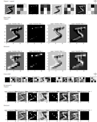

This ends the Convolutional Neural Networks from scratch part of the blog. There are many other algorithms done from scratch and available in this site too.