Multilayer Perceptron (MLP)
We all know that single layer perceptron are commonly used to classify problems that are linearly separable. If we choose a single layer perceptron for a non-linearly separable problem, the results may not be successful. As a result, we must look for an alternative solution to a non-linear problem, and one such solution is the multi layer perceptron. Because AND and OR problems are linearly separable, a single layer perceptron is adequate to solve them. However, the XOR problem cannot be solved by a single layer perceptron, thus we employed back propagation to solve it.
Back- Propagation
The back-propagation algorithm is a popular approach for training multi layer perceptrons. There are two stages to the training.
- Forward Phase
- Backward Phase
Forward Phase
The network's synaptic weights are fixed in this phase, and the input signal is propagated layer by layer through the network until it reaches the output. As a result, alterations in this phase are limited to the activation potentials and outputs of the network's neurons.
Backward Phase
An error signal is generated in this step by comparing the network's output to a desired response. The ensuing error signal is then propagated backwards, layer by layer, via the network. During the second phase, the network's synaptic weights are gradually adjusted.
Algorithm
forward algorithm is same as I wrote in single layer perceptron. Back propagation algorithm is given below.
-
The error signal at the output of neuron j at iteration n is given by
$$ e_j(n) = d_j(n) - y_j(n) $$ where dj(n) is actual output and yj(n) is predicted output By MLP -
The total error energy E(n) for all the neurons in the output layer is therefore
$$ E(n) = \frac{1}{2} \sum(e_j^2(n))$$
Where c is the set of neuron in the output layer.
-
Let N be the total number of training vectors (examples). Then the average squared error is
$$ E{avg} = \frac{1}{2} \sum{n=1}^{N} E(n) $$ -
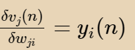
Consider the neuron j the local field vj(n) and output yj(n) of neuron j is given by
$$ vj(n) = \sum_{i=1}^{m} wji(n)yi(n) $$
$$ yj(n) = \phi_j(v_j(n))$$ where y_j is output of neuron i and w_ji is weight of link from i to j.
- The correction
$$
\Delta w_{ij}(n)$$
made to the weight is proportional to the partial derivative
$$
\frac{ \delta(E)}{\delta w_{ji}}$$
of instantaneous error
Using the chain rule of calculus, this gradient can be expressed as follows,
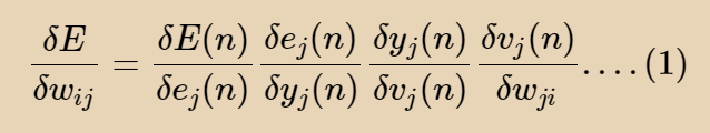
- We can get the following partial derivatives
$$ \frac{\delta E(n)}{\delta e_j(n)} = e_j(n)$$
$$ \frac{\delta e_j(n)}{\delta y_j(n)} = -1 $$
$$ \frac{\delta y_j(n)}{\delta v_j(n)} = \phi'_j(v_j(n))$$
Putting all partial derivatives in equation 1 we get,
$$
\frac{\delta E}{\delta w_{ij}} = - e_j(n)\phi'_j(v_j(n)) y_i(n).....(2)$$
Correction factor
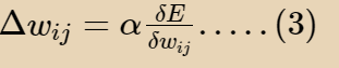
Using equation (2) and (3) we can write,
$$
\Delta w_{ij} = - \alpha e_j(n)\phi'_j(v_j(n)) y_i(n)......(4)$$
This can be written as,
$$ \delta w_{ij} = \alpha \delta y_j(n)$$ Where
$$ \delta_j(n) = e_j(n)\phi'_j(v_j(n))......(5)$$
- The error term in equation 4 and 5 depends upon location of neuron in the MLP.
Implementation of Multilayer perceptron From scratch
initialization of sigmoid function
# Training of XOR function using Backpropagation
import numpy as np
def sigmoid (x):
    return 1/(1 + np.exp(-x))
Sigmoid derivatives function
def sigmoid_derivative(x):
    return x * (1 - x)
We'll utilize the majority function in this case. Which works like this: if we have a grater number of zero, we get 0; similarly, if we have a grater number of one, we get 1.
given_input = np.array([[0,0,0],[0,0,1],[0,1,1],[0,1,0],[1,0,0],[1,0,1],[1,1,0],[1,1,1]])
expected_output = np.array([[0],[0],[1],[0],[0],[1],[1],[1]])
Set the epoch to the desired outcome and the learning parameter to the same value.
# initialization of epoch and learning rate
epochs = 10000
lr = 0.1
Here, we are going to use multilayer perceptron of size 3,2,2,1. That means 3 input node in input layer two hidden layers of size 2 and output layer.
# try differnet combinations
Input_LNeurons, Hidden_LNeurons1,Hidden_LNeurons2, Output_LNeurons = 3,2,2,1
Initialization of weight and bias for respective layer.
#Random weights and bias initialization
hidden_weight1 = np.random.uniform(size=(Input_LNeurons,Hidden_LNeurons1))

hidden_bias1 =np.random.uniform(size=(1,Hidden_LNeurons1))
hidden_weight2 = np.random.uniform(size=(Hidden_LNeurons1,Hidden_LNeurons2))

hidden_bias2 = np.random.uniform(size= (1,Hidden_LNeurons2))
output_weight = np.random.uniform(size=(Hidden_LNeurons2,Output_LNeurons))
output_bias = np.random.uniform(size=(1,Output_LNeurons))

print("middle hidden weights: ",end='')
print(*hidden_weight1)
print("Middle hidden bias: ",end='')
print(*hidden_bias1)
print("Final Hidden wights:",end ='')
print(hidden_weight2)
print("Final Hidden bias:", end = '')
print(hidden_bias2)
print("Final output weights: ",end='')
print(*output_weight)
print("Final output bias: ",end='')
print(*output_bias)
middle hidden weights: [0.33423001 0.4898466 ] [0.18806618 0.10893656] [0.10304258 0.19255168]
Middle hidden bias: [0.66140122 0.01344335]
Final Hidden wights:[[0.49194816 0.74464173]
[0.76910257 0.6362092 ]]
Final Hidden bias:[[0.35349949 0.47628357]]
Final output weights: [0.63626356] [0.80786521]
Final output bias: Forward training,
for i in range(epochs):
    hidden_layer_activation1 = np.dot(given_input, hidden_weight1)
    hidden_layer_activation1 += hidden_bias1
    hidden_layer_output1 = sigmoid(hidden_layer_activation1)

    hidden_layer_activation2 = np.dot(hidden_layer_output1,hidden_weight2)
    hidden_layer_activation2 += hidden_bias2
    hidden_layer_output2 = sigmoid(hidden_layer_activation2)

    output_activation = np.dot(hidden_layer_output2, output_weight)
    output_activation += output_bias
    predicted_output = sigmoid(output_activation)
Backward training can be done into two ways
Case I: Neuron j is output layer neuron
The neuron j's desired response dj(n) is directly available. In this example, calculating the error ej(n) is trivial. To determine the weight update term, we can utilize equations 4 or 5.
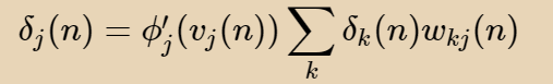
Case II: Neuron j is hidden layer neuron
Neuron j does not have any desirable responses. A hidden neuron's error signal must be calculated recursively in terms of the error signals of all neurons connected to it, as shown below.
for i in range(epochs):
    hidden_layer_activation1 = np.dot(given_input, hidden_weight1)
    hidden_layer_activation1 += hidden_bias1
    hidden_layer_output1 = sigmoid(hidden_layer_activation1)

    hidden_layer_activation2 = np.dot(hidden_layer_output1,hidden_weight2)
    hidden_layer_activation2 += hidden_bias2
    hidden_layer_output2 = sigmoid(hidden_layer_activation2)

    output_activation = np.dot(hidden_layer_output2, output_weight)
    output_activation += output_bias
    predicted_output = sigmoid(output_activation)

    error = expected_output - predicted_output
    d_predicted_output = error * sigmoid_derivative(predicted_output)

    error_hidden_layer2 = d_predicted_output.dot(output_weight.T)

    d_hidden_layer2 = error_hidden_layer2 * sigmoid_derivative(hidden_layer_output2)
    error_hidden_layer1 = d_hidden_layer2.dot(hidden_weight2.T)#hidden_error)
    d_hidden_layer1 = error_hidden_layer1 * sigmoid_derivative(hidden_layer_output1)

    output_weight += hidden_layer_output2.T.dot(d_predicted_output) *lr
    output_bias += np.sum(d_predicted_output,axis=0,keepdims=True) *lr
    hidden_weight2 += hidden_layer_output1.T.dot(d_hidden_layer2) * lr
    hidden_bias2 += np.sum(d_hidden_layer2,axis = 0, keepdims=True)*lr
    hidden_weight1 += x.T.dot(d_hidden_layer1)*lr
    hidden_bias1 += np.sum(d_hidden_layer1,axis=0,keepdims=True) *lr

print("nOutput from neural network after 10,000 epochs: ",end='')
print(*predicted_output)
print(*t)
Output from neural network after 10,000 epochs: [0.00803129] [0.02090726] [0.98338774] [0.02096907] [0.02100865] [0.98341657] [0.9834612] [0.99474155]
[0] [0] [1] [0] [0] [1] [1] [1]